


Software To Help You Turn Your Data Into AI
Forget fragmented workflows, annotation tools, and Notebooks for building AI applications. Encord Data Engine accelerates every step of taking your model into production.

Labeling and annotating images is easy. Video annotation is not. Too many platforms focus on image annotation, throwing in video as an additional suite of features rather than implementing video-native tools for annotators.
In this post, we outline the 5 features you need to maximize video annotation ROI and efficiencies so you can choose the right video annotation tool for your needs.
Video annotation is not the same as image annotation. You need a completely different — specialist, video-centric — a suite of tools and features to handle videos.
Otherwise, data and video analyst teams are juggling multiple annotation platforms (which is something we see more often than you’d imagine) to achieve their objectives.
As a leader or manager within an organization that needs a video annotation and labeling solution, you must ensure that the platform can effectively handle the specificities of video and image annotation.
For example, within a large video — with a long runtime — you need to ensure the correct coordinates of objects that move from one frame to the next are aligned with the frame and timestamp the object first appeared.
For several reasons, this doesn’t always happen with other tools, forcing companies to discard months’ worth of incorrectly labeled data. Let’s review the five most important features you need when considering which video annotation tool/platform to use.
Video annotation comes with dozens of challenges, such as variable frame rates, ghost frames, frame synchronization issues, and numerous others. To avoid these issues and ensure you don’t lose days of labeling activity, there are two things your video annotation platform needs:
Effective pre-processing solves these challenges, ensuring a video is displayed properly and ready for annotation. Pre-processing means you avoid needing to re-label everything if there’s an issue with the video (e.g., sync frame issues, video not displayed properly, annotations are not matched with the proper frames, etc.), saving your annotation team countless hours and a lot of budgets at the start of a project.
An easy-to-use video annotation and labeling interface ensures that annotators are productive. Video labeling and annotation shouldn’t take months, especially when annotating long videos. With this in mind, here are the key features you need to look out for to ensure your chosen annotation tool is easy to use:
Navigation features in the video annotation section of Encord
Another important feature of a great video annotation tool is the ability to classify frames and events. This gives you additional data for your model to work from - whether it was nighttime in the video or what the labeled object was doing at the time.
Dynamic classifications are often called action or “event-based” classifications. The clue is in the name - they tell you what the object is doing - whether the car that you’re tracking is turning from left to right over a specific number of frames; hence these classifications are dynamic. It depends on what’s going on in the video and the granular level of detail you need to label. Dynamic or event-based classifications are a powerful feature that the best video annotation platforms come with, and you can use them regardless of the annotation type used to originally label the object in motion.
Frame Classifications are different from specific object classifications. Instead of labeling or classifying an object, you use an annotation tool to organize a specific frame within a video. Hotkeys and video labeling menus can make it simple to select the start and end of a frame and then give that frame a label while annotating. A frame classification is used to highlight something happening in the frame itself - whether it is day or night or raining or sunny, for example.
Annotation is a time-consuming, manual, data-intensive task. Especially when videos are long, complicated, or there are hundreds of videos to annotate. A solution is to automate video annotations.
Automation leverages the skills of your annotation teams. It saves time and money while increasing the efficiency and the quality of the annotation work.
For example, if an annotator has drawn a label boundary around a specific object — e.g., a cellular cluster being analyzed — the goal of auto-object segmentation is to tighten the edges so it fits more closely around the image in question. Algorithms can also track this image throughout the video automatically.
Example of automated labeling using interpolation in Encord
Large annotation teams are difficult to manage. Whether you’re a Head of Machine Learning or Data Operations leader, you’ve got to juggle team management, budgets, operational timelines, and project outputs.
Project leaders need visibility on what’s going on, being processed, and being analyzed. You need a clear understanding of the state of the project in real-time, giving you the ability to react fast if anything changes.
When big-budget and long-timescale annotation projects are underway, it’s often useful to leverage external annotation teams to implement labor-intensive aspects of the project.
But working with external providers creates the need for advanced team and project management features, such as:
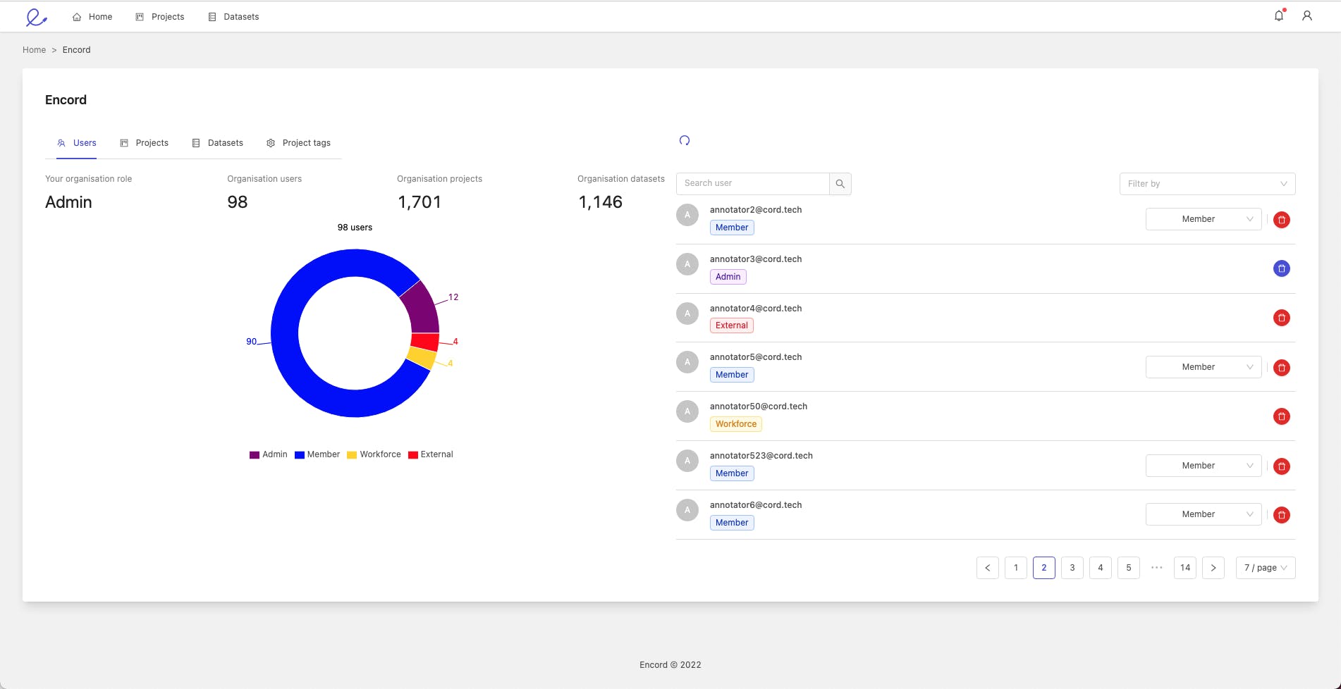
User management in Encord
And there we go, the 5 features every video annotation tool needs.
At Encord, our active learning platform for computer vision is used by a wide range of sectors - including healthcare, manufacturing, utilities, and smart cities - to annotate videos and accelerate their computer vision model development.
Experience Encord in action. Dramatically reduce manual video annotation tasks, generating massive savings and efficiencies. Try it for free today.


Join the Encord Developers community to discuss the latest in computer vision, machine learning, and data-centric AI
Join the communityRelated Blogs

What is a Data Lake? A data lake is a centralized repository where you can store all your structured, semi-structured, and unstructured data types at any scale for processing, curation, and analytics. It supports batch and real-time streams to combine raw data from diverse sources (databases, IoT devices, mobile apps, etc.) into the repository without a predefined schema. It has been 12 years since the New York Times published an interesting article on ‘The Age of Big Data,’ in which most of the talk and tooling were centered around analytics. Fast-forward to today, and we are continuously grappling with the influx of data at the petabyte (PB) and zettabyte (ZB) scales, which is getting increasingly complex in dimensions (images, videos, point cloud data, etc.). It is clear that solutions that can help manage the size and complexity of data are needed for organizational success. This has urged data, AI, and technology teams to look towards three pivotal data management solutions: data lakes, data warehouses, and cloud services. This article focuses on understanding data lakes as a data management solution for machine learning (ML) teams. You will learn: What a data lake is and how it differs from a data warehouse. Benefits and limitations of a data lake for ML teams. The data lake architecture. Best practices for setting up a data lake. On-premise vs. cloud-based data lakes. Computer vision use cases of data lakes. TL; DR A data lake is a centralized repository for diverse, structured, and unstructured data. Key architecture components include Data Sources, Data Ingestion, Data Persistence and Storage, Data Processing Layer, Analytical Sandboxes, Data Lake Zones, and Data Consumption. Best practices for data lakes involve defining clear objectives, robust data governance, scalability, prioritizing security, encouraging a data-driven culture, and quality control. On-premises data lakes offer control and security; cloud-based data lakes provide scalability and cost efficiency. Data lakes are evolving with advanced analytics and computer vision use cases, emphasizing the need for adaptable systems and adopting forward-thinking strategies. Overview: Data Warehousing, Data Lake, and Cloud Storage Data Warehouses A data warehouse is a single location where an organization's structured data is consolidated, transformed, and stored for query and analysis. The structured data is ideal for generating reports and conducting analytics that inform business decisions. Limitations Limited agility in handling unstructured or semi-structured data. Can create data silos, hindering cross-departmental data sharing. Data Lakes A data lake stores vast amounts of raw datasets in their native format until needed, which includes structured, semi-structured, and unstructured data. This flexibility supports diverse applications, from computer vision use cases to real-time analytics. Challenges Risk of becoming a "data swamp" if not properly managed, with unclear, unclean, or redundant data. Requires robust metadata and governance practices to ensure data is findable and usable. Cloud Storage and Computing Cloud computing encompasses a broad spectrum of services beyond storage, such as processing power and advanced analytics. Cloud storage refers explicitly to storing data on the internet through a cloud computing provider that manages and operates data storage as a service. Risks Security concerns, requiring stringent data access controls and encryption. Potential for unexpected costs if usage is not monitored. Dependence on the service provider's reliability and continuity. Data lake overview with the data being ingested from different sources. Most ML teams misinterpret the role of data lakes and data warehouses, choosing an inappropriate management solution. Before delving into the rest of the article, let’s clarify how they differ. Data Lake vs. Data Warehouse Understanding the strengths and use cases of data lakes and warehouses can help your organization maximize its data assets. This can help create an efficient data infrastructure that supports various analytics, reporting, and ML needs. Let’s compare a data lake to a data warehouse based on specific features. Choosing Between Data Lake and Data Warehouse The choice between a data lake and a warehouse depends on the specific needs of the analysis. For an e-commerce organization analyzing structured sales data, a data warehouse offers the speed and efficiency required for such tasks. However, a data lake (or a combination of both solutions) might be more appropriate for applications that require advanced computer vision (CV) techniques and large visual datasets (images, videos). Benefits of a Data Lake Data lakes offer myriad benefits to organizations using complex datasets for analytical insights, ML workloads, and operational efficiency. Here's an overview of the key benefits: Single Source of Truth: When you centralize data in data lakes, you get rid of data silos, which makes data more accessible across the whole organization. So, data lakes ensure that all the data in an organization is consistent and reliable by providing a single source of truth. Schema on Read: Unlike traditional databases that define data structure at write time (schema on write), data lakes allow the structure to be imposed at read time to offer flexibility in data analysis and utilization. Scalability and Cost-Effectiveness: Data lakes' cloud-based nature facilitates scalable storage solutions and computing resources, optimizing costs by reducing data duplication. Decoupling of Storage and Compute: Data lakes let different programs access the same data without being dependent on each other. This makes the system more flexible and helps it use its resources more efficiently. Architectural Principles for Data Lake Design When designing a data lake, consider these foundational principles: Decoupled Architecture: Data ingestion, processing, curation, and consumption should be independent to improve system resilience and adaptability. Tool Selection: Choose the appropriate tools and platforms based on data characteristics, ingestion, and processing requirements, avoiding a one-size-fits-all approach. Data Temperature Awareness: Classify data as hot (frequently accessed), warm (less frequently accessed), or cold (rarely accessed but retained for compliance) to optimize storage strategies and access patterns based on usage frequency. Leverage Managed Services: Use managed or serverless services to reduce operational overhead and focus on value-added activities. Immutability and Event Journaling: Design data lakes to be immutable, preserving historical data integrity and supporting comprehensive data analysis. They should also store and version the data labels. Cost-Conscious Design: Implement strategies (balancing performance, access needs, budget constraints) to manage and optimize costs without compromising data accessibility or functionality. Data Lake Architecture A robust data lake architecture is pivotal for harnessing the power of large datasets so organizations can store, process, and analyze them efficiently. This architecture typically comprises several layers dedicated to a specific function within the data management ecosystem. Below is an overview of these key components: Data Sources Diverse Producers: Data lakes can ingest data from a myriad of sources, including, but not limited to, IoT devices, cameras, weblogs, social media, mobile apps, transactional databases (SQL, NoSQL), and external APIs. This inclusivity enables a holistic view of business operations and customer interactions. Multiple Formats: They accommodate a wide range of data formats, from structured data in CSVs and databases to unstructured data like videos, images, DICOM files, documents, and multimedia files, providing a unified repository for all organizational data. This, of course, does not exclude semi-structured data like XML and JSON files. Data Ingestion Batch and Streaming: Data ingestion mechanisms in a data lake architecture support batch and real-time data flows. Use tools and services to auto-ingest the data so the system can effectively capture it. Validation and Metadata: Data is tagged with metadata during ingestion for easy retrieval, and initial validation checks are performed to ensure data quality and integrity. Data Governance Zone Access Control and Auditing: Implementing robust access controls, encryption, and auditing capabilities ensures data security and privacy, crucial for maintaining trust and compliance. Metadata Management: Documenting data origins, formats, lineage, ownership, and usage history is central to governance. This component incorporates tools for managing metadata, which facilitates data discovery, lineage tracking, and cataloging, enhancing the usability and governance of the data lake. Data Persistence and Staging Raw Data Storage: Data is initially stored in a staging area in raw, unprocessed form. This approach ensures that the original data is preserved for future processing needs and compliance requirements. Staging Area: Data may be staged or temporarily held in a dedicated area within the lake before processing. To efficiently handle the volume and variety of data, this area is built on scalable storage technologies, such as HDFS (Hadoop Distributed File System) or cloud-based storage services like Amazon S3. Data Processing Layer Transformation and Enrichment: This layer transforms data into a more usable format, often involving data cleaning, enrichment, deduplication, anonymization, normalization, and aggregation processes. It also improves data quality and ensures reliability for downstream analysis. Processing Engines: To cater to various processing needs, the architecture should support multiple processing engines, such as Hadoop for batch processing, Spark for in-memory processing, and others for specific tasks like stream processing. Data Indexing: This component indexes processed data to facilitate faster search and retrieval. It is crucial for supporting efficient data exploration and curation. Related: Interested in learning the techniques and best data cleaning and preprocessing practices? Check out one of our most-read guides, “Mastering Data Cleaning & Data Preprocessing.” Data Quality Monitoring Continuous Quality Checks: Implements automated processes for continuous monitoring of data quality, identifying issues like inconsistencies, duplications, or anomalies to maintain the accuracy, integrity, and reliability of the data lake. Quality Metrics and Alerts: Define and track data quality metrics, set up alert mechanisms for when data quality thresholds are breached, and enable proactive issue resolution. Related: Read how you can automate the assessment of training data quality in this article. Analytical Sandboxes Exploration and Experimentation: Computer vision engineers and data scientists can use analytical sandboxes to experiment with data sets, build models, and visually explore data (e.g., images, videos) and embeddings without impacting the integrity of the primary data (versioned data and labels). Tool Integration: These sandboxes support a wide range of analytics, data, and ML tools, giving users the flexibility and choice to work with their preferred technologies. Worth Noting: Building computer vision applications? Encord Active integrates with Annotate (with cloud platform integrations) and provides explorers with a way to explore image embeddings for any scale of data visually. See how to use it in the docs. Data Consumption Access and Integration: Data stored in the data lake is accessible to various downstream applications and users, including BI tools, reporting systems, computer vision platforms, or custom applications. This accessibility ensures that insights from the data lake can drive decision-making across the organization. APIs and Data Services: For programmatic access, APIs and data services enable developers and applications to query and retrieve data from the data lake, integrating data-driven insights into business processes and applications. Best Practices for Setting Up a Data Lake Implementing a data lake requires careful consideration and adherence to best practices to be successful and sustainable. Here are some suggested best practices to help you set up a data lake that can grow with your organization’s changing and growing data needs: #1. Define Clear Objectives and Scope Understand Your Data Needs: Before setting up a data lake, identify the types of data you plan to store, the insights you aim to derive, and the stakeholders who will consume this data. This understanding will guide your data lake's design, architecture, and governance model. Set Clear Objectives: Establish specific, measurable objectives for your data lake, such as improving data accessibility for analytics, supporting computer vision projects, or consolidating disparate data sources. These objectives will help prioritize features and guide decision-making throughout the setup process. #2. Ensure Robust Data Governance Implement a Data Governance Framework: A strong governance framework is essential for maintaining data quality, managing access controls, and ensuring compliance with regulatory standards. This framework should include data ingestion, storage, management, and archival policies. Metadata Management: Cataloging data with metadata is crucial for making it discoverable (indexing, filtering, sorting) and understandable. Implement tools and processes to automatically capture metadata, including data source, tags, format, and access permissions, during ingestion or at rest. Metadata can be technical (data design; schema, tables, formats, source documentation), business (docs on usage), and operational (events, access history, trace logs). #3. Focus on Scalability and Flexibility Choose Scalable Infrastructure: Whether on-premises or cloud-based, ensure your data lake infrastructure can scale to accommodate future data growth without significant rework or additional investment. Plan for Varied Data Types: Design your data lake to handle structured, semi-structured, and unstructured data. Flexibility in storing and processing different data types (images, videos, DICOM, blob files, etc.) ensures the data lake can support a wide range of use cases. #4. Prioritize Security and Compliance Implement Strong Security Measures: Security is paramount for protecting sensitive data and maintaining user trust. Apply encryption in transit and at rest, manage access with role-based controls, and regularly audit data access and usage. Compliance and Data Privacy: Consider the legal and regulatory requirements relevant to your data. Incorporate compliance controls into your data lake's architecture and operations, including data retention policies and the right to be forgotten. #5. Foster a Data-Driven Culture Encourage Collaboration: Promote collaboration between software engineers, CV engineers, data scientists, and analysts to ensure the data lake meets the diverse needs of its users. Regular feedback loops can help refine and enhance the data lake's utility. Education and Training: Invest in stakeholder training to maximize the data lake's value. Understanding how to use the data lake effectively can spur innovation and lead to new insights across the organization. #6. Continuous Monitoring and Optimization Monitor Data Lake Health: Regularly monitor the data lake for performance, usage patterns, and data quality issues. This proactive approach can help identify and resolve problems before they impact users. Iterate and Optimize: Your organization's needs will evolve, and so will your data lake. Continuously assess its performance and utility, adjusting based on user feedback and changing business requirements. Cloud-based Data Lake Platforms Cloud-based data lake platforms offer scalable, flexible, and cost-effective solutions for storing and analyzing large amounts of data. These platforms provide Data Lake as a Service (DLaaS), which simplifies the setup and management of data lakes. This allows organizations to focus on deriving insights rather than infrastructure management. Let's explore the architecture of data lake platforms provided by AWS, Azure, Snowflake, GCP, and their applications in multi-cloud environments. AWS Data Lake Architecture Amazon Web Services (AWS) provides a comprehensive and mature set of services to build a data lake. The core components include: Ingestion: AWS Glue for ETL processes and AWS Kinesis for real-time data streaming. Storage: Amazon S3 for scalable and secure data storage. Processing and Analysis: Amazon EMR is used for big data processing, AWS Glue for data preparation and loading, and Amazon Redshift for data warehousing. Consumption: Send your curated data to AWS SageMaker to run ML workloads or Amazon QuickSight to build visualizations, perform ad-hoc analysis, and quickly get business insights from data. Security and Governance: AWS Lake Formation automates the setup of a secure data lake, manages data access and permissions, and provides a centralized catalog for discovering and searching for data. Azure Data Lake Architecture Azure's data lake architecture is centered around Azure Data Lake Storage (ADLS) Gen2, which combines the capabilities of Azure Blob Storage and ADLS Gen1. It offers large-scale data storage with a hierarchical namespace and a secure HDFS-compatible data lake. Ingestion: Azure Data Factory for ETL operations and Azure Event Hubs for real-time event processing. Storage: ADLS Gen2 for a highly scalable data lake foundation. Processing and Consumption: Azure Databricks for big data analytics running on Apache Spark, Azure Synapse Analytics for querying (SQL serverless) and analysis (Notebooks), and Azure HDInsight for Hadoop-based services. Power BI can connect to ADLS Gen2 directly to create interactive reports and dashboards. Security and Governance: Azure provides fine-grained access control with Azure Role-Based Access Control (RBAC) and secures data with Microsoft Entra ID. Snowflake Data Lake Architecture Snowflake's unique architecture separates compute and storage, allowing users to scale them independently. It offers a cloud-agnostic solution operating across AWS, Azure, and GCP. Ingestion: Within Snowflake, Snowpipe Streaming runs on top of Apache Kafka for real-time ingestion. Apache Kafka acts as the messaging broker between the source and Snowlake. You can run batch ingestion with Python scripts and the PUT command. Storage: Uses cloud provider's storage (S3, ADLS, or Google Cloud Storage) or internal (i.e., Snowflake) stages to store structured, unstructured, and semi-structured data in their native format. Processing and Curation: Snowflake's Virtual Warehouses provide dedicated compute resources for data processing for high performance and concurrency. Snowpark can implement business logic within existing programming languages. Data Sharing and Governance: Snowflake enables secure data sharing between Snowflake accounts with governance features for managing data access and security. Consumption: Snowflake provides native connectors for popular BI and data visualization tools, including Google Analytics and Looker. Snowflake Marketplace provides users access to a data marketplace to discover and access third-party data sets and services. Snowpark helps with features for end-to-end ML. High-level architecture for running data lake workloads using Snowpark in Snowflake Google Cloud Data Lake Architecture In addition to various processing and analysis services, Google Cloud Platform (GCP) bases its data lake solutions on Google Cloud Storage (GCS), the primary data storage service. Ingestion: Cloud Pub/Sub for real-time messaging Storage: GCS offers durable and highly available object storage. Processing: Cloud Data Fusion offers pre-built transformations for batch and real-time processing, and Dataflow is for serverless stream and batch data processing. Consumption and Analysis: BigQuery provides serverless, highly scalable data analysis with an SQL-like interface. Dataproc runs Apache Hadoop and Spark jobs. Vertex AI provides machine learning capabilities to analyze and derive insights from lake data. Security and Governance: Cloud Identity and Access Management (IAM) controls resource access, and Cloud Data Loss Prevention (DLP) helps discover and protect sensitive data. Data Lake Architecture on Multi-Cloud Multi-cloud data lake architectures leverage services from multiple cloud providers, optimizing for performance, cost, and regulatory compliance. This approach often involves: Cloud-Agnostic Storage Solutions: Storing data in a manner accessible across cloud environments, either through multi-cloud storage services or by replicating data across cloud providers. Cross-Cloud Services Integration: This involves using best-of-breed services from different cloud providers for ingestion, processing, analysis, and governance, facilitated by data integration and orchestration tools. Unified Management and Governance: Implement multi-cloud management platforms to ensure consistent monitoring, security, and governance across cloud environments. Implementing a multi-cloud data lake architecture requires careful planning and robust data management strategies to ensure seamless operation, data consistency, and compliance across cloud boundaries. On-Premises Data Lakes and Cloud-based Data Lakes Organizations looking to implement data lakes have two primary deployment models to consider: on-premises and cloud-based (although more recent approaches involve a hybrid of both solutions). Cost, scalability, security, and accessibility affect each model's advantages and disadvantages. On-Premises Data Lakes: Advantages Control and Security: On-premises data lakes offer organizations complete control over their infrastructure, which can be crucial for industries with stringent regulatory and compliance requirements. This control also includes data security, so security measures can be tailored to each organization's needs. Performance: With data stored locally, on-premises solutions can provide faster data access and processing speeds, which is beneficial for time-sensitive applications that require rapid data retrieval and analysis. On-Premises Data Lakes: Challenges Cost and Scalability: Establishing an on-premises data lake requires a significant upfront investment in hardware and infrastructure. Scaling up can also require additional hardware purchases and be time-consuming. Maintenance: On-premises data lakes necessitate ongoing maintenance, including hardware upgrades, software updates, and security patches, which require dedicated IT staff and resources. Cloud-based Data Lakes: Advantages Scalability and Flexibility: Cloud-based data lakes can change their storage and computing power based on changing data volumes and processing needs without changing hardware. Cost Efficiency: A pay-as-you-go pricing model allows organizations to avoid substantial upfront investments and only pay for their storage and computing resources, potentially reducing overall costs. Innovative Features: Cloud service providers always add new technologies and features to their services, giving businesses access to the most advanced data management and analytics tools. Cloud-based Data Lakes: Challenges Data Security and Privacy: While cloud providers implement robust security measures, organizations may have concerns about storing sensitive data off-premises, particularly in industries with strict data sovereignty regulations. Dependence on Internet Connectivity: Access to cloud-based data lakes relies on stable internet connectivity. Any disruptions in connectivity can affect data access and processing, impacting operations. Understanding these differences enables organizations to select the most appropriate data lake solution to support their data management strategy and business objectives. Computer Vision Use Cases of Data Lakes Data lakes are pivotal in powering computer vision applications across various industries by providing a scalable repository for storing and analyzing vast large image and video datasets in real-time. Here are some compelling use cases where data lakes improve computer vision applications: Healthcare: Medical Imaging and Diagnosis In healthcare, data lakes store vast collections of medical images (e.g., X-rays, MRIs, CT scans, PET) that, combined with data curation tools, can improve image quality, detect anomalies, and provide quantitative assessments. CV algorithms analyze these images in real time to diagnose diseases, monitor treatment progress, and plan surgeries. Case Study: Viz.ai uses artificial intelligence to speed care and improve patient outcomes. In this case study, learn how they ingest, annotate, curate, and consume medical data. Autonomous Vehicles: Navigation and Safety Autonomous vehicle developers use data lakes to ingest and curate diverse datasets from vehicle sensors, including cameras, LiDAR, and radar. This data is crucial for training computer vision algorithms that enable autonomous driving capabilities, such as object detection, automated curb management, traffic sign recognition, and pedestrian tracking. Case Study: Automotus builds real-time curbside management automation solutions. Learn how they ingested raw, unlabeled data into Encord via Annotate and curated a balanced, diverse dataset with Active in this case study. How Automotus increased mAP 20% by reducing their dataset size by 35% with visual data curation Agriculture: Precision Farming In the agricultural sector, data lakes store and curate visual data (images and videos) captured by drones or satellites over farmland. Computer vision techniques analyze this data to assess crop health, identify pest infestations, and evaluate water usage, so farmers can make informed decisions and apply treatments selectively. Case Study: Automated harvesting and analytics company Four Growers uses Encord’s platform and annotators to help build its training datasets from scratch, labeling millions of instances of greenhouses and plants. Learn how the platform has halved the time it takes for them to build training data in this case study. Security and Surveillance: Threat Detection Government and private security agencies use data lakes to compile video feeds from CCTV cameras in public spaces, airports, and critical infrastructure. Real-time analysis with computer vision helps detect suspicious activities, unattended objects, and unauthorized entries, triggering immediate responses to potential security threats. ML Team's Data Lake Guide: Key Takeaways Data lakes have become essential for scalable storage and processing of diverse data types in modern data management. They facilitate advanced analytics, including real-time applications like computer vision. Their ability to transform sectors ranging from finance to agriculture by enhancing operational efficiencies and providing actionable insights makes them invaluable. As we look ahead: The continuous evolution of data lake architectures, especially within cloud-native and multi-cloud contexts, promises to bring forth advanced tools and services for improved data handling. This progression presents an opportunity for enterprises to transition from viewing data lakes merely as data repositories to leveraging them as strategic assets capable of building advanced CV applications. To maximize data lakes, address the problems associated with data governance, security, and quality. This will ensure that data remains a valuable organizational asset and a catalyst for data-driven decision-making and strategy formulation.
March 28
11 min

Dimensionality reduction is a fundamental technique in machine learning (ML) that simplifies datasets by reducing the number of input variables or features. This simplification is crucial for enhancing computational efficiency and model performance, especially as datasets grow in size and complexity. High-dimensional datasets, often comprising hundreds or thousands of features, introduce the "curse of dimensionality." This effect slows down algorithms by making data scarceness (sparsity) and computing needs grow exponentially. Dimensionality reduction changes the data into a simpler, lower-dimensional space that is easier to work with while keeping its main features. This makes computation easier and lowers the risk of overfitting. This strategy is increasingly indispensable in the era of big data, where managing vast volumes of information is a common challenge. This article provides insight into various approaches, from classical methods like principal component analysis (PCA) and linear discriminant analysis (LDA) to advanced techniques such as manifold learning and autoencoders. Each technique has benefits and works best with certain data types and ML problems. This shows how flexible and different dimensionality reduction methods are for getting accurate and efficient model performance when dealing with high-dimensional data. Here are the Twelve (12) techniques you will learn in this article: Manifold Learning (t-SNE, UMAP) Principal Component Analysis (PCA) Independent Component Analysis (ICA) Sequential Non-negative Matrix Factorization (NMF) Linear Discriminant Analysis (LDA) Generalized Discriminant Analysis (GDA) Missing Values Ratio (MVR): Threshold Setting Low Variance Filter High Correlation Filter Forward Feature Construction Backward Feature Elimination Autoencoders Classification of Dimensionality Reduction Techniques Dimensionality reduction techniques preserve important data, make it easier to use in other situations, and speed up learning. They do this using two steps: feature selection, which preserves the most important variables, and feature projection, which creates new variables by combining the original ones in a big way. Feature Selection Techniques Techniques classified under this category can identify and retain the most relevant features for model training. This approach helps reduce complexity and improve interpretability without significantly compromising accuracy. They are divided into: Embedded Methods: These integrate feature selection within model training, such as LASSO (L1) regularization, which reduces feature count by applying penalties to model parameters and feature importance scores from Random Forests. Filters: These use statistical measures to select features independently of machine learning models, including low-variance filters and correlation-based selection methods. More sophisticated filters involve Pearson’s correlation and Chi-Squared tests to assess the relationship between each feature and the target variable. Wrappers: These assess different feature subsets to find the most effective combination, though they are computationally more demanding. Feature Projection Techniques Feature projection transforms the data into a lower-dimensional space, maintaining its essential structures while reducing complexity. Key methods include: Manifold Learning (t-SNE, UMAP). Principal Component Analysis (PCA). Kernel PCA (K-PCA). Linear Discriminant Analysis (LDA). Quadratic Discriminant Analysis (QDA). Generalized Discriminant Analysis (GDA). 1. Manifold Learning Manifold learning, a subset of non-linear dimensionality reduction techniques, is designed to uncover the intricate structure of high-dimensional data by projecting it into a lower-dimensional space. Understanding Manifold Learning At the heart of Manifold Learning is that while data may exist in a high-dimensional space, the intrinsic dimensionality—representing the true degrees of freedom within the data—is often much lower. For example, images of faces, despite being composed of thousands of pixels (high-dimensional data points), might be effectively described with far fewer dimensions, such as the angles and distances between key facial features. Core Techniques and Algorithms t-Distributed Stochastic Neighbor Embedding (t-SNE): t-SNE is powerful for visualizing high-dimensional data in two or three dimensions. It converts similarities between data points to joint probabilities and minimizes the divergence between them in different spaces, excelling in revealing clusters within data. Uniform Manifold Approximation and Projection (UMAP): UMAP is a relatively recent technique that balances the preservation of local and global data structures for superior speed and scalability. It's computationally efficient and has gained popularity for its ability to handle large datasets and complex topologies. Isomap (Isometric Mapping): Isomap extends classical Multidimensional Scaling (MDS) by incorporating geodesic distances among points. It's particularly effective for datasets where the manifold (geometric surface) is roughly isometric to a Euclidean space, allowing global properties to be preserved. Locally Linear Embedding (LLE): LLE reconstructs high-dimensional data points from their nearest neighbors, assuming the manifold is locally linear. By preserving local relationships, LLE can unfold twisted or folded manifolds. t-SNE and UMAP are two of the most commonly applied dimensionality reduction techniques. At Encord, we use UMAP to generate the 2D embedding plots in Encord Active. 2. Principal Component Analysis (PCA) The Principal Component Analysis (PCA) algorithm is a method used to reduce the dimensionality of a dataset while preserving as much information (variance) as possible. As a linear reduction method, PCA transforms a complex dataset with many variables into a simpler one that retains critical trends and patterns. What is variance? Variance measures the data spread around the mean, and features with low variance indicate little variation in their values. These features often need to be more formal for subsequent analysis and can hinder model performance. What is Principal Component Analysis (PCA)? PCA identifies and uses the principal components (directions that maximize variance and are orthogonal to each other) to effectively project data into a lower-dimensional space. This process begins with standardizing the original variables, ensuring their equal contribution to the analysis by normalizing them to have a zero mean and unit variance. Step-by-Step Explanation of Principal Component Analysis Standardization: Normalize the data so each variable contributes equally, addressing PCA's sensitivity to variable scales. Covariance Matrix Computation: Compute the covariance matrix to understand how the variables of the input dataset deviate from the mean and to see if they are related (i.e., correlated). Finding Eigenvectors and Eigenvalues: Find the new axes (eigenvectors) that maximize variance (measured by eigenvalues), making sure they are orthogonal to show that variance can go in different directions. Sorting and Ranking: Prioritize eigenvectors (and thus principal components) by their ability to capture data variance, using eigenvalues as the metric of importance. Feature Vector Formation: Select a subset of eigenvectors based on their ranking to form a feature vector. This subset of eigenvectors forms the principal components. Transformation: Map the original data into this principal component space, enabling analysis or further machine learning in a more tractable, less noisy space. Dimensionality reduction using PCA Applications PCA is widely used in exploratory data analysis and predictive modeling. It is also applied in areas like image compression, genomics for pattern recognition, and financial data for uncovering latent patterns and correlations. PCA can help visualize complex datasets by reducing data dimensionality. It can also make machine learning algorithms more efficient by reducing computational costs and avoiding overfitting with high-dimensional data. 3. Independent Component Analysis (ICA) Independent Component Analysis (ICA) is a computational method in signal processing that separates a multivariate signal into additive, statistically independent subcomponents. Statistical independence is critical because Gaussian variables maximize entropy given a fixed variance, making non-Gaussianity a key indicator of independence. Originating from the work of Hérault and Jutten in 1985, ICA excels in applications like the "cocktail party problem," where it isolates distinct audio streams amid noise without prior source information. Example of the cocktail party problem The cocktail party problem involves separating original sounds, such as music and voice, from mixed signals recorded by two microphones. Each microphone captures a different combination of these sounds due to its varying proximity to the sound sources. ICA is distinct from methods like PCA because it focuses on maximizing statistical independence between components rather than merely de-correlating them. Principles Behind Independent Component Analysis The essence of ICA is its focus on identifying and separating independent non-Gaussian signals embedded within a dataset. It uses the fact that these signals are statistically independent and non-Gaussian to divide the mixed signals into separate parts from different sources. This demixing process is pivotal, transforming seemingly inextricable data (impossible to separate) into interpretable components. Two main strategies for defining component independence in ICA are the minimization of mutual information and non-Gaussianity maximization. Various algorithms, such as infomax, FastICA, and kernel ICA, implement these strategies through measures like kurtosis and negentropy. Algorithmic Process To achieve its goals, ICA incorporates several preprocessing steps: Centering adjusts the data to have a zero mean, ensuring that analyses focus on variance rather than mean differences. Whitening transforms the data into uncorrelated variables, simplifying the subsequent separation process. After these steps, ICA applies iterative methods to separate independent components, and it often uses auxiliary methods like PCA or singular value decomposition (SVD) to lower the number of dimensions at the start. This sets the stage for efficient and robust component extraction. By breaking signals down into basic, understandable parts, ICA provides valuable information and makes advanced data analysis easier, which shows its importance in modern signal processing and beyond. Let’s see some of its applications. Applications of ICA The versatility of ICA is evident across various domains: In telecommunications, it enhances signal clarity amidst interference. Finance benefits from its ability to identify underlying factors in complex market data, assess risk, and detect anomalies. In biomedical signal analysis, it dissects EEG or fMRI data to isolate neurological activity from artifacts (such as eye blinks). 4. Sequential Non-negative Matrix Factorization (NMF) Nonnegative matrix Factorization (NMF) is a technique in multivariate analysis and linear algebra in which a matrix V is factorized into two lower-dimensional matrices, W (basis matrix) and H (coefficient matrix), with the constraint that all matrices involved have no negative elements. This factorization works especially well for fields where the data is naturally non-negative, like genetic expression data or audio spectrograms, because it makes it easy to understand the parts. The primary aim of NMF is to reduce dimensionality and uncover hidden/latent structures in the data. Principle of Sequential Non-negative Matrix Factorization The distinctive aspect of Sequential NMF is its iterative approach to decomposing matrix V into W and H, making it adept at handling time-series data or datasets where the temporal evolution of components is crucial. This is particularly relevant in dynamic datasets or applications where data evolves. Sequential NMF responds to changes by repeatedly updating W and H, capturing changing patterns or features important in online learning, streaming data, or time-series analysis. In text mining, for example, V denotes a term-document matrix over time, where W represents evolving topics and H indicates their significance across different documents or time points. This dynamic representation allows the monitoring of trends and changes in the dataset's underlying structure. Procedure of feature extraction using NMF Applications The adaptability of Sequential NMF has led to its application in a broad range of fields, including: Medical Research: In oncology, Sequential NMF plays a pivotal role in analyzing genetic data over time, aiding in the classification of cancer types, and identifying temporal patterns in biomarker expression. Audio Signal Processing: It is used to analyze sequences of audio signals and capture the temporal evolution of musical notes or speech. Astronomy and Computer Vision: Sequential NMF tracks and analyzes the temporal changes in celestial bodies or dynamic scenes. 5. Linear Discriminant Analysis (LDA) Linear Discriminant Analysis (LDA) is a supervised machine learning technique used primarily for pattern classification, dimensionality reduction, and feature extraction. It focuses on maximizing class separability. Unlike PCA, which optimizes for variance regardless of class labels, LDA aims to find a linear combination of features that separates different classes. It projects data onto a lower-dimensional space using class labels to accomplish this. Imagine, for example, a dataset of two distinct groups of points spread in space; LDA aims to find a projection where these groups are as distinct as possible, unlike PCA, which would look for the direction of highest variance regardless of class distinction. This method is highly efficient in scenarios where the division between categories of data is to be accentuated. PCA Vs. LDA: What's the Difference? Assumptions of LDA Linear Discriminant Analysis (LDA) operates under assumptions essential for effectively classifying observations into predefined groups based on predictor variables. These assumptions, elaborated below, play a critical role in the accuracy and reliability of LDA's predictions. Multivariate Normality: Each class must follow a multivariate normal distribution (multi-dimensional bell curve). You can asses this through visual plots or statistical tests before applying LDA. Homogeneity of Variances (Homoscedasticity): Ensuring uniform variance across groups helps maintain the reliability of LDA's projections. Techniques like Levene's test can assess this assumption. Absence of Multicollinearity: LDA requires predictors to be relatively independent. Techniques like variance inflation factors (VIFs) can diagnose multicollinearity issues. Working Methodology of Linear Discriminant Analysis LDA transforms the feature space into a lower-dimensional one that maximizes class separability by: Calculating mean vectors for each class. Computing within-class and between-class scatter matrices to understand the distribution and separation of classes. Solving for the eigenvalues and eigenvectors that maximize the between-class variance relative to the within-class variance. This defines the optimal projection space to distinguish the classes. Tools like Python's Scikit-learn library simplify applying LDA with functions specifically designed to carry out these steps efficiently. Applications LDA's ability to reduce dimensionality while preserving as much of the class discriminatory information as possible makes it a powerful feature extraction and classification tool applicable across various domains. Examples: In facial recognition, LDA enhances the distinction between individual faces to improve recognition accuracy. Medical diagnostics benefit from LDA's ability to classify patient data into distinct disease categories, aiding in early and accurate diagnosis. In marketing, LDA helps segment customers for targeted marketing campaigns based on demographic and behavioral data. 6. Generalized Discriminant Analysis (GDA) Generalized Discriminant Analysis (GDA) extends linear discriminant analysis (LDA) into a nonlinear domain. It uses kernel functions to project input data vectors into a higher-dimensional feature space to capture complex patterns that LDA, limited to linear boundaries, might miss. These functions project data into a higher-dimensional space where inseparable classes in the original space can be distinctly separated. Step-by-step Explanation of Generalized Discriminant Analysis The core objective of GDA is to find a low-dimensional projection that maximizes the between-class scatter while minimizing the within-class scatter in the high-dimensional feature space. Let’s examine the GDA algorithm step by step: 1. Kernel Function Selection: First, choose an appropriate kernel function (e.g., polynomial, radial basis function (RBF)) that transforms the input data into a higher-dimensional space. 2. Kernel Matrix Computation: Compute the kernel matrix K, representing the high-dimensional dot products between all pairs of data points. This matrix is central to transforming the data into a feature space without explicitly performing the computationally expensive mapping. 3. Scatter Matrix Calculation in Feature Space: In the feature space, compute the within-class scatter matrix SW and the between-class scatter matrix SB, using the kernel matrix K to account for the data's nonlinear transformation. 4. Eigenvalue Problem: Solving this problem in the feature space identifies the projection vectors that best separate the classes by maximizing the SB/SW ratio. This step is crucial for identifying the most informative projections for class separation. 5. Projection: Use the obtained eigenvectors to project the input data onto a lower-dimensional space that maximizes class separability to achieve GDA's goal of improved class recognition. Applications GDA has been applied in various domains, benefiting from its ability to handle nonlinear patterns: Image and Video Recognition: GDA is used for facial recognition, object detection, and activity recognition in videos, where the data often exhibit complex, nonlinear relationships. Biomedical Signal Processing: In analyzing EEG, ECG signals, and other biomedical data, GDA helps distinguish between different physiological states or diagnose diseases. Text Classification and Sentiment Analysis: GDA transforms text data into a higher-dimensional space, effectively separating documents or sentiments that are not linearly separable in the original feature space. 7. Missing Values Ratio (MVR): Threshold Setting Datasets often contain missing values, which can significantly impact the effectiveness of dimensionality reduction techniques. One approach to addressing this challenge is to utilize a missing values ratio (MVR) thresholding technique for feature selection. Process of Setting Threshold for Missing Values The MVR for a feature is calculated as the percentage of missing values for data points. The optimal threshold is dependent on several factors, including the dataset’s nature and the intended analysis: Determining the Threshold: Use statistical analyses, domain expertise, and exploratory data analysis (e.g., histograms of missing value ratios) to identify a suitable threshold. This decision balances retaining valuable data against excluding features that could introduce bias or noise. Implications of Threshold Settings: A high threshold may retain too many features with missing data, complicating the analysis. Conversely, a low threshold could lead to excessive data loss. Regularly, thresholds between 20% to 60% are considered, but this range varies widely based on the data context and analysis goals. Contextual Considerations: The dataset's specific characteristics and the chosen dimensionality reduction technique influence the threshold setting. Methods sensitive to data sparsity or noise may require a lower MVR threshold. Example: In a dataset with 100 observations, a feature with 75 missing values has an MVR of 75%. If the threshold is set at 70%, this feature would be considered for removal. Applications High-throughput Biological Data Analysis: Technical limitations often render Gene expression data incomplete. Setting a conservative MVR threshold may preserve crucial biological insights by retaining genes with marginally incomplete data. Customer Data Analysis: Customer surveys may have varying completion rates across questions. MVR thresholding identifies which survey items provide the most complete and reliable data, sharpening customer insights. Social Media Analysis: Social media data can be sparse, with certain users' entries missing. MVR thresholding can help select informative features for user profiling or sentiment analysis. 8. Low Variance Filter A low variance filter is a straightforward preprocessing technique aimed at reducing dimensionality by eliminating features with minimal variance, focusing analysis on more informative aspects of the dataset. Steps for Implementing a Low Variance Filter Calculate Variance: For each feature in the dataset, compute the variance. Prioritize scaling or normalizing data to ensure variance is measured on a comparable basis across all features. Set Threshold: Define a threshold for the minimum acceptable variance. This threshold often depends on the specific dataset and analysis objectives but typically ranges from a small percentage of the total variance observed across features. Feature Selection: Exclude features with variances below the threshold. Tools like Python's `pandas` library or R's `caret` package can efficiently automate this process. Applications of Low Variance Filter Across Domains Sensor Data Analysis: Sensor readings might exhibit minimal fluctuation over time, leading to features with low variance. Removing these features can help focus on the sensor data's more dynamic aspects. Image Processing: Images can contain features representing background noise. These features often have low variance and can be eliminated using the low variance filter before image analysis. Text Classification: Text data might contain stop words or punctuation marks that offer minimal information for classification. The low variance filter can help remove such features, improving classification accuracy. 9. High Correlation Filter The high correlation filter is a crucial technique for addressing feature redundancy. Eliminating highly correlated features optimizes datasets for improved model accuracy and efficiency. Steps for Implementing a High Correlation Filter Compute Correlation Matrix: Assess the relationship between all feature pairs using an appropriate correlation coefficient, such as Pearson for continuous features (linear relationships) and Spearman for ordinal (monotonic relationships). Define Threshold: Establish a correlation coefficient threshold above highly correlated features. A common threshold of 0.8 or 0.9 may vary based on specific model requirements and data sensitivity. Feature Selection: Identify sets of features whose correlation exceeds the threshold. From each set, retain only one feature based on criteria like predictive power, data completeness, or domain relevance and remove the others. Applications Financial Data Analysis: Stock prices or other financial metrics might exhibit a high correlation, often reflecting market trends. The high correlation filter can help select a representative subset of features for financial modeling. Bioinformatics: Gene expression data can involve genes with similar functions, leading to high correlation. Selecting a subset of uncorrelated genes can be beneficial for identifying distinct biological processes. Recommendation Systems: User profiles often contain correlated features like similar purchase history or browsing behavior. The high correlation filter can help select representative features to build more efficient recommendation models. While the Low Variance Filter method removes features with minimal variance, discarding data points that likely don't contribute much information, the High Correlation Filter approach identifies and eliminates highly correlated features. This process is crucial because two highly correlated features carry similar information, increasing redundancy within the model. 10. Forward Feature Construction Forward Feature Construction (FFC) is a methodical approach to feature selection, designed to incrementally build a model by adding features that offer the most significant improvement. This technique is particularly effective when the relationship between features and the target variable is complex and needs to be fully understood. Algorithm for Forward Feature Construction Initiate with a Null Model: Start with a baseline model without any predictors to establish a performance benchmark. Evaluation Potential Additions: For each candidate feature outside the model, assess potential performance improvements by adding that feature. Select the Best Feature: Incorporate the feature that significantly improves performance. Ensure the model remains interpretable and manageable. Iteration: Continue adding features until further additions fail to offer significant gains, considering computational efficiency and the risk of diminishing returns. Practical Considerations and Implementation Performance Metrics: To gauge improvements, use appropriate metrics, such as the Akaike Information Criterion (AIC) for regression or accuracy and the F1 score for classification, adapting the choice of metric to the model's context. Challenges: Be mindful of computational demands and the potential for multicollinearity. Implementing strategies to mitigate these risks, such as pre-screening features or setting a cap on the number of features, can be crucial. Tools: Leverage software tools and libraries (e.g., R's `stepAIC` or Python's `mlxtend.SequentialFeatureSelector`) that support efficient FFC application and streamline feature selection. Applications of FFC Across Domains Clinical Trials Prediction: In clinical research, FFC facilitates the identification of the most predictive biomarkers or clinical variables from a vast dataset, optimizing models for outcome prediction. Financial Modeling: In financial market analysis, this method distills a complex set of economic indicators down to a core subset that most accurately forecasts market movements or financial risk. 11. Backward Feature Elimination Backward Feature Elimination (BFE) systematically simplifies machine learning models by iteratively removing the least critical features, starting with a model that includes the entire set of features. This technique is particularly suited for refining linear and logistic regression models, where dimensionality reduction can significantly improve performance and interpretability. Algorithm for Backward Feature Elimination Initialize with Full Model: Construct a model incorporating all available features to establish a comprehensive baseline. Identify and Remove Least Impactful Feature: Determine the feature whose removal least affects or improves the model's predictive performance. Use metrics like p-values or importance scores to eliminate it from the model. Performance Evaluation: After each removal, assess the model to ensure performance remains robust. Utilize cross-validation or similar methods to validate performance objectively. Iterative Optimization: Continue this evaluation and elimination process until further removals degrade model performance, indicating that an optimal feature subset has been reached. Learn how to validate the performance of your ML model in this guide to validation model performance with Encord Active. Practical Considerations for Implementation Computational Efficiency: Given the potentially high computational load, especially with large feature sets, employ strategies like parallel processing or stepwise evaluation to simplify the Backward Feature Elimination (BFE) process. Complex Feature Interactions: Special attention is needed when features interact or are categorical. Consider their relationships to avoid inadvertently removing significant predictors. Applications Backward Feature Elimination is particularly useful in contexts like: Genomics: In genomics research, BFE helps distill large datasets into a manageable number of significant genes to improve understanding of genetic influences on diseases. High-dimensional Data Analysis: BFE simplifies complex models in various fields, from finance to the social sciences, by identifying and eliminating redundant features. This could reduce overfitting and improve the model's generalizability. While Forward Feature Construction is beneficial for gradually building a model by adding one feature at a time, Backward Feature Elimination is advantageous for models starting with a comprehensive set of features and needing to identify redundancies. 12. Autoencoders Autoencoders are a unique type of neural network used in deep learning, primarily for dimensionality reduction and feature learning. They are designed to encode inputs into a compressed, lower-dimensional form and reconstruct the output as closely as possible to the original input. This process emphasizes the encoder-decoder structure. The encoder reduces the dimensionality, and the decoder attempts to reconstruct the input from this reduced encoding. How Does Autoencoders Work? They achieve dimensionality reduction and feature learning by mimicking the input data through encoding and decoding. 1. Encoding: Imagine a bottle with a narrow neck in the middle. The data (e.g., an image) is the input that goes into the wide top part of the bottle. The encoder acts like this narrow neck, compressing the data into a smaller representation. This compressed version, often called the latent space representation, captures the essential features of the original data. The encoder is typically made up of multiple neural network layers that gradually reduce the dimensionality of the data. The autoencoder learns to discard irrelevant information and focus on the most important characteristics by forcing the data through this bottleneck. 2. Decoding: Now, imagine flipping the bottle upside down. The decoder acts like the wide bottom part, trying to recreate the original data from the compressed representation that came through the neck. The decoder also uses multiple neural network layers, but this time, it gradually increases the data's dimensionality, aiming to reconstruct the original input as accurately as possible. Variants and Advanced Applications Sparse Autoencoders: Introduce regularization terms to enforce sparsity in the latent representation, enhancing feature selection. Denoising Autoencoders: Specifically designed to remove noise from data, these autoencoders learn to recover clean data from noisy inputs, offering superior performance in image and signal processing tasks. Variational Autoencoders (VAEs): VAEs make new data samples possible by treating the latent space as a probabilistic distribution. This opens up new ways to use generative modeling. Training Nuances Autoencoders use optimizers like Adam or stochastic gradient descent (SGD) to improve reconstruction accuracy by improving their weights through backpropagation. Overfitting prevention is integral and can be addressed through methods like dropout, L1/L2 regularization, or a validation set for early stopping. Applications Autoencoders have a wide range of applications, including but not limited to: Dimensionality Reduction: Similar to PCA but more powerful (as non-linear alternatives), autoencoders can perform non-linear dimensionality reductions, making them particularly useful for preprocessing steps in machine learning pipelines. Image Denoising: By learning to map noisy inputs to clean outputs, denoising autoencoders can effectively remove noise from images, surpassing traditional denoising methods in efficiency and accuracy. Generative modeling: Variational autoencoders (VAEs) can make new data samples similar to the original input data by modeling the latent space as a continuous probability distribution. (e.g., Generative Adversarial Networks (GANs)). Impact of Dimensionality Reduction in Smart City Solutions Automotus is a company at the forefront of using AI to revolutionize smart city infrastructure, particularly traffic management. They achieve this by deploying intelligent traffic monitoring systems that capture vast amounts of video data from urban environments. However, efficiently processing and analyzing this high-dimensional data presents a significant challenge. This is where dimensionality reduction techniques come into play. The sheer volume of video data generated by Automotus' traffic monitoring systems necessitates dimensionality reduction techniques to make data processing and analysis manageable. PCA identifies the most significant features in the data (video frames in this case) and transforms them into a lower-dimensional space while retaining the maximum amount of variance. This allows Automotus to extract the essential information from the video data, such as traffic flow patterns, vehicle types, and potential congestion points, without analyzing every pixel. Partnering with Encord, Automotus led to a 20% increase in model accuracy and a 35% reduction in dataset size. This collaboration focused on dimensionality reduction, leveraging Encord Annotate’s flexible ontology, quality control capabilities, and automated labeling features. That approach helped Automotus reduce infrastructure constraints, improve model performance to provide better data to clients, and reduce labeling costs. Efficiency directly contributes to Automotus's business growth and operational scalability. The team used Encord Active to visually inspect, query, and sort their datasets to remove unwanted and poor-quality data with just a few clicks, leading to a 35% reduction in the size of the datasets for annotation. This enabled the team to cut their labeling costs by over a third. Interested in learning more? Read the full story on Encord's website for more details. Dimensionality Reduction Technique: Key Takeaways Dimensionality reduction techniques simplify models and enhance computational efficiency. They help manage the "curse of dimensionality," improving model generalizability and reducing overfitting risk. These techniques are used for feature selection and extraction, contributing to better model performance. They are applied in various fields, such as image and speech recognition, financial analysis, and bioinformatics, showcasing their versatility. By reducing the number of input variables, these methods ensure models are computationally efficient and capture essential data patterns for more accurate predictions.
March 22
10 min

In computer vision, you cannot overstate the importance of data quality. It directly affects how accurate and reliable your models are. This guide is about understanding why high-quality data matters in computer vision and how to improve your data quality. We will explore the essential aspects of data quality and its role in model accuracy and reliability. We will discuss the key steps for improving quality, from selecting the right data to detecting outliers. We will also see how Encord Active helps us do all this to improve our computer vision models. This is an in-depth guide; feel free to use the table of contents on the left to navigate each section and find one that interests you. By the end, you’ll have a solid understanding of the essence of data quality for computer vision projects and how to improve it to produce high-quality models. Let’s dive right into it! Introduction to Data Quality in Computer Vision Defining the Attributes of High-Quality Data High-quality data includes several attributes that collectively strengthen the robustness of computer vision models: Accuracy: Precision in reflecting real-world objects is vital; inaccuracies can lead to biases and diminished performance. Consistency: Uniformity in data, achieved through standardization, prevents conflicts and aids effective generalization. Data Diversity: By incorporating diverse data, such as different perspectives, lighting conditions, and backgrounds, you enhance the model's adaptability, making it resilient to potential biases and more adept at handling unforeseen challenges. Relevance: Data curation should filter irrelevant data, ensuring the model focuses on features relevant to its goals. Ethical Considerations: Data collected and labeled ethically, without biases, contributes to responsible and fair computer vision models. By prioritizing these data attributes, you can establish a strong foundation for collecting and preparing quality data for your computer vision projects. Next, let's discuss the impact of these attributes on model performance. Impact of Data Quality on Model Performance Here are a few aspects of high-quality data that impact the model's performance: Accuracy Improvement: Curated and relevant datasets could significantly improve model accuracy. Generalization Capabilities: High-quality data enables models to apply learned knowledge to new, unseen scenarios. Increased Model Robustness: Robust models are resilient to variations in input conditions, which is perfect for production applications. As we explore enhancing data quality for training computer vision models, it's essential to underscore that investing in data quality goes beyond mere accuracy. It's about constructing a robust and dependable system. By prioritizing clean, complete, diverse, and representative data, you establish the foundation for effective models. Considerations for Training Computer Vision Models Training a robust computer vision model hinges significantly on the training data's quality, quantity, and labeling. Here, we explore the key considerations for training CV models: Data Quality The foundation of a robust computer vision model rests on the quality of its training data. Data quality encompasses the accuracy, completeness, reliability, and relevance of the information within the dataset. Addressing missing values, outliers, and noise is crucial to ensuring the data accurately reflects real-world scenarios. Ethical considerations, like unbiased representation, are also paramount in curating a high-quality dataset. Data Diversity Data diversity ensures that the model encounters many scenarios. Without diversity, models risk being overly specialized and may struggle to perform effectively in new or varied environments. By ensuring a diverse dataset, models can better generalize and accurately interpret real-world situations, improving their robustness and reliability. Data Quantity While quality takes precedence, an adequate volume of data is equally vital for comprehensive model training. Sufficient data quantity contributes to the model's ability to learn patterns, generalize effectively, and adapt to diverse situations. The balance of quality and quantity ensures a holistic learning experience for the model, enabling it to navigate various scenarios. It's also important to balance the volume of data with the model's capacity and computational efficiency to avoid issues like overfitting and unnecessary computational load. Label Quality The quality of its labels greatly influences the precision of a computer vision model. Consistent and accurate labeling with sophisticated annotation tools is essential for effective training. Poorly labeled data can lead to biases and inaccuracies, undermining the model's predictive capabilities. Read How to Choose the Right Data for Your Computer Vision Project to learn more about it. Data Annotation Tool A reliable data annotation tool is equally essential to ensuring high-quality data. These tools facilitate the labeling of images, improving the quality of the data. By providing a user-friendly interface, efficient workflows, and diverse annotation options, these tools streamline the process of adding valuable insights to the data. Properly annotated data ensures the model receives accurate ground truth labels, significantly contributing to its learning process and overall performance. Selecting the Right Data for Your Computer Vision Projects The first step in improving data quality is data curation. This process involves defining criteria for data quality and establishing mechanisms for sourcing reliable datasets. Here are a few key steps to follow when selecting the data for your computer vision project: Criteria for Selecting Quality Data The key criteria for selecting high-quality data include: Accuracy: Data should precisely reflect real-world scenarios to avoid biases and inaccuracies. Completeness: Comprehensive datasets covering diverse situations are crucial for generalization. Consistency: Uniformity in data format and preprocessing ensures reliable model performance. Timeliness: Regular updates maintain relevance, especially in dynamic or evolving environments. Evaluating and Sourcing Reliable Data The process of evaluating and selecting reliable data involves: Quality Metrics: Validating data integrity through comprehensive quality metrics, ensuring accuracy, completeness, and consistency in the dataset. Ethical Considerations: Ensuring data is collected and labeled ethically without introducing biases. Source Reliability: Assessing and selecting trustworthy data sources to mitigate potential biases. Case Studies: Improving Data Quality Improved Model Performance by 20% When faced with challenges managing and converting vast amounts of images into labeled training data, Autonomous turned to Encord. The flexible ontology structure, quality control capabilities, and automated labeling features of Encord were instrumental in overcoming labeling obstacles. The result was twofold: improved model performance and economic efficiency. With Encord, Autonomous efficiently curated and reduced the dataset by getting rid of data that was not useful. This led to a 20% improvement in mAP (mean Average Precision), a key metric for measuring the accuracy of object detection models. This was not only effective in addressing the accuracy of the model but also in reducing labeling costs. Efficient data curation helped prioritize which data to label, resulting in a 33% reduction in labeling costs. Thus, improving the accuracy of the models enhanced the quality of the data that Autonomous delivered to its customers. Read the case study on how Automotus increased mAP by 20% by reducing their dataset size by 35% with visual data curation to learn more about it. Following data sourcing, the next step involves inspecting the quality of the data. Let's learn how to explore data quality with Encord Active. Exploring Data Quality using Encord Active Encord Active provides a comprehensive set of tools to evaluate and improve the quality of your data. It uses quality metrics to assess the quality of your data, labels, and model predictions. Data Quality Metrics analyzes your images, sequences, or videos. These metrics are label-agnostic and depend only on the image content. Examples include image uniqueness, diversity, area, brightness, sharpness, etc. Label Quality Metrics operates on image labels like bounding boxes, polygons, and polylines. These metrics can help you sort data, filter it, find duplicate labels, and understand the quality of your annotations. Examples include border proximity, broken object tracks, classification quality, label duplicates, object classification quality, etc. Read How to Detect Data Quality Issues in a Torchvision Dataset Using Encord Active for a more comprehensive insight. In addition to the metrics that ship with Encord Active, you can define custom quality metrics for indexing your data. This allows you to customize the evaluation of your data according to your specific needs. Here's a step-by-step guide to exploring data quality through Encord Active: Create an Encord Active Project Initiating your journey with Encord Active begins with creating a project in Annotate, setting the foundation for an efficient and streamlined data annotation process. Follow these steps for a curation workflow from Annotate to Active: Create a Project in Annotate. Add an existing dataset or create your dataset. Set up the ontology of the annotation project. Customize the workflow design to assign tasks to annotators and for expert review. Start the annotation process! Read the documentation to learn how to create your annotation project on Encord Annotate. Import Encord Active Project Once you label a project in Annotate, transition to Active by clicking Import Annotate Project. Read the documentation to learn how to import your Encord Annotate project to Encord Active Cloud. Using Quality Metrics After choosing your project, navigate to Filter on the Explorer page >> Choose a Metric from the selection of data quality metrics to visually analyze the quality of your dataset. Great! That helps you identify potential issues such as inconsistencies, outliers, etc., which helps make informed decisions regarding data cleaning. Guide to Data Cleaning Data cleaning involves identifying and rectifying errors, inconsistencies, and inaccuracies in datasets. This critical phase ensures that the data used for computer vision projects is reliable, accurate, and conducive to optimal model performance. Understanding Data Cleaning and Its Benefits Data cleaning involves identifying and rectifying data errors, inconsistencies, and inaccuracies. The benefits include: Improved Data Accuracy: By eliminating errors and inconsistencies, data cleaning ensures that the dataset accurately represents real-world phenomena, leading to more reliable model outcomes. Increased Confidence in Model Results: A cleaned dataset instills confidence in the reliability of model predictions and outputs. Better Decision-Making Based on Reliable Data: Organizations can make better-informed decisions to build more reliable AI. Read How to Clean Data for Computer Vision to learn more about it. Selecting the right tool is essential for data cleaning tasks. In the next section, you will see criteria for selecting data cleaning tools to automate repetitive tasks and ensure thorough and efficient data cleansing. Selecting a Data Cleaning Tool Some criteria for selecting the right tools for data cleaning involve considering the following: Diversity in Functionality: Assess whether the tool specializes in handling specific data issues such as missing values or outlier detections. Understanding the strengths and weaknesses of each tool enables you to align them with the specific requirements of their datasets. Scalability and Performance: Analyzing the performance of tools in terms of processing speed and resource utilization helps in selecting tools that can handle the scale of the data at hand efficiently. User-Interface and Accessibility: Tools with intuitive interfaces and clear documentation streamline the process, reducing the learning curve. Compatibility and Integration: Compatibility with existing data processing pipelines and integration capabilities with popular programming languages and platforms are crucial. Seamless integration ensures a smooth workflow, minimizing disruptions during the data cleaning process. Once a suitable data cleaning tool is selected, understanding and implementing best practices for effective data cleaning becomes imperative. These practices ensure you can optimally leverage the tool you choose to achieve desired outcomes. Best Practices for Effective Data Cleaning Adhering to best practices is essential for ensuring the success of the data cleaning process. Some key practices include: Data Profiling: Understand the characteristics and structure of the data before initiating the cleaning process. Remove Duplicate and Irrelevant Data: Identify and eliminate duplicate or irrelevant images/videos to ensure data consistency and improve model training efficiency. Anomaly Detection: Utilize anomaly detection techniques to identify outliers or anomalies in image/video data, which may indicate data collection or processing errors. Documentation: Maintain detailed documentation of the cleaning process, including the steps taken and the rationale behind each decision. Iterative Process: Treat data cleaning as an iterative process, revisiting and refining as needed to achieve the desired data quality. For more information, read Mastering Data Cleaning & Data Preprocessing. Overcoming Challenges in Image and Video Data Cleaning Cleaning image and video data presents unique challenges compared to tabular data. Issues such as noise, artifacts, and varying resolutions require specialized techniques. These challenges need to be addressed using specialized tools and methodologies to ensure the accuracy and reliability of the analyses. Visual Inspection Tools: Visual data often contains artifacts, noise, and anomalies that may not be immediately apparent in raw datasets. Utilizing tools that enable visual inspection is essential. Platforms allowing users to view images or video frames alongside metadata provide a holistic understanding of the data. Metric-Based Cleaning: Implementing quantitative metrics is equally vital for effective data cleaning. You can use metrics such as image sharpness, color distribution, blur, and object recognition accuracy to identify and address issues. Tools that integrate these metrics into the cleaning process automate the identification of outliers and abnormalities, facilitating a more objective approach to data cleaning. Using tools and libraries streamlines the cleaning process and contributes to improved insights and decision-making based on high-quality visual data. Watch the webinar From Data to Diamonds: Unearth the True Value of Quality Data to learn how tools help. Using Encord Active to Clean the Data Let’s take an example of the COCO 2017 dataset imported to Encord Active. Upon analyzing the dataset, Encord Active highlights both severe and moderate outliers. While outliers bear significance, maintaining a balance is crucial. Using Filter, Encord Active empowers users to visually inspect outliers and make informed decisions regarding their inclusion in the dataset. Taking the Area metric as an example, it reveals numerous severe outliers. We identify 46 low-resolution images with filtering, potentially hindering effective training for object detection. Consequently, we can select the dataset, click Add to Collection, remove these images from the dataset, or export them for cleaning with a data preprocessing tool. Encord Active facilitates visual and analytical inspection, allowing users to detect datasets for optimal preprocessing. This iterative process ensures the data is of good quality for the model training stage and improves performance on computer vision tasks. Watch the webinar Big Data to Smart Data Webinar: How to Clean and Curate Your Visual Datasets for AI Development to learn how to use tools to efficiently curate your data.. Case Studies: Optimizing Data Cleaning for Self-Driving Cars with Encord Active Encord Active (EA) streamlines the data cleaning process for computer vision projects by providing quality metrics and visual inspection capabilities. In a practical use case involving managing and curating data for self-driving cars, Alex, a DataOps manager at self-dr-AI-ving, uses Encord Active's features, such as bulk classification, to identify and curate low-quality annotations. These functionalities significantly improve the data curation process. The initial setup involves importing images into Active, where the magic begins. Alex organizes data into collections, an example being the "RoadSigns" Collection, designed explicitly for annotating road signs. Alex then bulk-finds traffic sign images using the embeddings and similarity search. Alex then clicks Add to a Collection, then Existing Collection, and adds the images to the RoadSigns Collection. Alex categorizes the annotations for road signs into good and bad quality, anticipating future actions like labeling or augmentation. Alex sends the Collection of low-quality images to a new project in Encord Annotate to re-label the images. After completing the annotation, Alex syncs the Project data with Active. He heads back to the dashboard and uses the model prediction analytics to gain insights into the quality of annotations. Encord Active's integration and efficient workflows empower Alex to focus on strategic tasks, providing the self-driving team with a streamlined and improved data cleaning process that ensures the highest data quality standards. Data Preprocessing What is Data Preprocessing? Data preprocessing transforms raw data into a format suitable for analysis. In computer vision, this process involves cleaning, organizing, and using feature engineering to extract meaningful information or features. Feature engineering helps algorithms better understand and represent the underlying patterns in visual data. Data preprocessing addresses missing values, outliers, and inconsistencies, ensuring that the image or video data is conducive to accurate analyses and optimal model training. Data Cleaning Vs. Data Preprocessing: The Difference Data cleaning involves identifying and addressing issues in the raw visual data, such as removing noise, handling corrupt images, or correcting image errors. This step ensures the data is accurate and suitable for further processing. Data preprocessing includes a broader set of tasks beyond cleaning, encompassing operations like resizing images, normalizing pixel values, and augmenting data (e.g., rotating or flipping images). The goal is to prepare the data for the specific requirements of a computer vision model. Techniques for Robust Data Preprocessing Image Standardization: Adjusting images to a standardized size facilitates uniform processing. Cropping focuses on relevant regions of interest, eliminating unnecessary background noise. Normalization: Scaling pixel values to a consistent range (normalization) and ensuring a standardized distribution enhances model convergence during training. Data Augmentation: Introduces variations in training data, such as rotations, flips, and zooms, and enhances model robustness. Data augmentation helps prevent overfitting and improves the model's generalization to unseen data. Dealing with Missing Data: Addressing missing values in image datasets involves strategies like interpolating or generating synthetic data to maintain data integrity. Noise Reduction: Applying filters or algorithms to reduce image noise, such as blurring or denoising techniques, enhances the clarity of relevant information. Color Space Conversion: Converting images to different color spaces (e.g., RGB to grayscale) can simplify data representation and reduce computational complexity. Now that we've laid the groundwork with data preprocessing, let's explore how to further elevate model performance through data refinement. Enhancing Models with Data Refinement Unlike traditional model-centric approaches, data refinement represents a paradigm shift, emphasizing nuanced and effective data-centric strategies. This approach empowers practitioners to leverage the full potential of their models through informed data selection and precise labeling, fostering a continuous cycle of improvement. By emphasizing input data refinement, you can develop a dataset that optimally aligns with the model's capabilities and enhances its overall performance. Model-centric vs Data-centric Approaches Model-Centric Approach: Emphasizes refining algorithms and optimizing model architectures. This approach is advantageous in scenarios where computational enhancements can significantly boost performance. Data-Centric Approach: Prioritizes the quality and relevance of training data. It’s often more effective when data quality is the primary bottleneck in achieving higher model accuracy. The choice between these approaches often hinges on the specific challenges of a given task and the available resources for model development. Download the free whitepaper How to Adopt a Data-Centric AI to learn how to make your AI strategy data-centric and improve performance. Data Refinement Techniques: Active Learning and Semi-Supervised Learning Active Learning: It is a dynamic approach that involves iteratively selecting the most informative data points for labeling. For example, image recognition might prioritize images where the model's predictions are most uncertain. This method optimizes labeling efforts and enhances the model's learning efficiency. Semi-Supervised Learning: It tackles scenarios where acquiring labeled data is challenging. This technique combines labeled and unlabeled data for training, effectively harnessing the potential of a broader dataset. For instance, in a facial recognition task, a model can learn general features from a large pool of unlabeled faces and fine-tune its understanding with a smaller set of labeled data. With our focus on refining data for optimal model performance, let's now turn our attention to the task of identifying and addressing outliers to improve the quality of our training data. Improving Training Data with Outlier Detection Outlier detection is an important step in refining machine learning models. Outliers, or abnormal data points, have the potential to distort model performance, making their identification and management essential for accurate training. Understanding Outlier Detection Outliers, or anomalous data points, can significantly impact the performance and reliability of machine learning models. Identifying and handling outliers is crucial to ensuring the training data is representative and conducive to accurate model training. Outlier detection involves identifying data points that deviate significantly from the expected patterns within a dataset. These anomalies can arise due to errors in data collection, measurement inaccuracies, or genuine rare occurrences. For example, consider a scenario where an image dataset for facial recognition contains rare instances with extreme lighting conditions or highly distorted faces. Detecting and appropriately addressing these outliers becomes essential to maintaining the model's robustness and generalization capabilities. Implementing Outlier Detection with Encord Active The outlier detection feature in Encord Active is robust. It can find and label outliers using predefined metrics, custom metrics, label classes, and pre-calculated interquartile ranges. It’s a systematic approach to debugging your data. This feature identifies data points that deviate significantly from established norms. In a few easy steps, you can efficiently detect outliers: Accessing Data Quality Metrics: Navigate to the Analytics > Data tab within Encord Active. Quality metrics offer a comprehensive overview of your dataset. In a practical scenario, a data scientist working on traffic image analysis might use Encord Active to identify and examine atypical images, such as those with unusual lighting conditions or unexpected objects, ensuring these don’t skew the model’s understanding of standard traffic scenes. Read the blog Improving Training Data with Outlier Detection to learn how to use Encord Active for efficient outlier detection. Understanding and Identifying Imbalanced Data Addressing imbalanced data is crucial for developing accurate and unbiased machine learning models. An imbalance in class distribution can lead to models that are skewed towards the majority class, resulting in poor performance in minority classes. Strategies for Achieving Balanced Datasets Resampling Techniques: Techniques like SMOTE for oversampling minority classes or Tomek Links for undersampling majority classes can help achieve balance. Synthetic Data Generation: Using data augmentation or synthetic data generation (e.g., GANs, generative models) to create additional examples for minority classes. Ensemble Methods: Implement ensemble methods that assign different class weights, enabling the model to focus on minority classes during training. Cost-Sensitive Learning: Adjust the misclassification cost associated with minority and majority classes to emphasize the significance of correct predictions for the minority class. When thoughtfully applied, these strategies create balanced datasets, mitigate bias, and ensure models generalize well across all classes. Balancing Datasets Using Encord Active Encord Active can address imbalanced datasets for a fair representation of classes. Its features facilitate an intuitive exploration of class distributions to identify and rectify imbalances. Its functionalities enable class distribution analysis. Automated analysis of class distributions helps you quickly identify imbalance issues based on pre-defined or custom data quality metrics. For instance, in a facial recognition project, you could use Encord Active to analyze the distribution of different demographic groups within the dataset (custom metric). Based on this analysis, apply appropriate resampling or synthetic data generation techniques to ensure a fair representation of all groups. Understanding Data Drift in Machine Learning Models What is Data Drift? Data drift is the change in statistical properties of the data over time, which can degrade a machine learning model's performance. Data drift includes changes in user behavior, environmental changes, or alterations in data collection processes. Detecting and addressing data drift is essential to maintaining a model's accuracy and reliability. Strategies for Detecting and Addressing Data Drift Monitoring Key Metrics: Regularly monitor key performance metrics of your machine learning model. Sudden changes or degradation in metrics such as accuracy, precision, or recall may indicate potential data drift. Using Drift Detection Tools: Tools that utilize statistical methods or ML algorithms to compare current data with training data effectively identify drifts. Retraining Models: Implement a proactive retraining strategy. Periodically update your model using recent and relevant data to ensure it adapts to evolving patterns and maintains accuracy. Continuous Monitoring and Data Feedback: Establish a continuous monitoring and adaptation system. Regularly validate the model against new data and adjust its parameters or retrain it as needed to counteract the effects of data drift. Practical Implementation and Challenges Imagine an e-commerce platform that utilizes a computer vision-based recommendation system to suggest products based on visual attributes. This system relies on constantly evolving image data for products and user interaction patterns. Identifying and addressing data drift Monitoring User Interaction with Image Data: Regularly analyzing how users interact with product images can indicate shifts in preferences, such as changes in popular colors, styles, or features. Using Computer Vision Drift Detection Tools: Tools that analyze changes in image data distributions are employed. For example, a noticeable shift in the popularity of particular styles or colors in product images could signal a drift. Retraining the recommendation model Once a drift is detected, you must update the model to reflect current trends. This might involve retraining the model with recent images of products that have gained popularity or adjusting the weighting of visual features the model considers important. For instance, if users start showing a preference for brighter colors, the recommendation system is retrained to prioritize such products in its suggestions. The key is to establish a balance between responsiveness to drift and the practicalities of model maintenance. Read the blog How To Detect Data Drift on Datasets for more information. Next, let's delve into a practical approach to inspecting problematic images to identify and address potential data quality issues. Inspect the Problematic Images Encord Active provides a visual dataset overview, indicating duplicate, blurry, dark, and bright images. This accelerates identifying and inspecting problematic images for efficient data quality enhancement decisions. Use visual representations for quick identification and targeted resolution of issues within the dataset. Severe and Moderate Outliers In the Analytics section, you can distinguish between severe and moderate outliers in your image set, understand the degree of deviation from expected patterns, and address potential data quality concerns. For example, below is the dataset analysis of the COCO 2017 dataset. It shows the data outliers in each metric and their severity. Blurry Images in the Image Set The blurry images in the image set represent instances where the visual content lacks sharpness or clarity. These images may exhibit visual distortions or unfocused elements, potentially impacting the overall quality of the dataset. You can also use the filter to exclude blurry images and control the quantity of retained high-quality images in the dataset. Darkest Images in the Image Set The darkest images in the image set are those with the lowest overall brightness levels. Identifying and managing these images is essential to ensure optimal visibility and clarity within the dataset, particularly in scenarios where image brightness impacts the effectiveness of model training and performance analysis. Duplicate or Nearly Similar Images in the Set Duplicate or nearly similar images in the set are instances where multiple images exhibit substantial visual resemblance or share identical content. Identifying and managing these duplicates is important for maintaining dataset integrity, eliminating redundancy, and ensuring that the model is trained on diverse and representative data. Next Steps: Fixing Data Quality Issues Once you identify problematic images, the next steps involve strategic methods to enhance data quality. Encord Active provides versatile tools for targeted improvements: Re-Labeling Addressing labeling discrepancies is imperative for dataset accuracy. Use re-labeling to rectify errors and inconsistencies in low-quality annotation. Encord Active simplifies this process with its Collection feature, selecting images for easy organization and transfer back for re-labeling. This streamlined workflow enhances efficiency and accuracy in the data refinement process. Active Learning Leveraging active learning workflows to address data quality issues is a strategic move toward improving machine learning models. Active learning involves iteratively training a model on a subset of data it finds challenging or uncertain. This approach improves the model's understanding of complex patterns and improves predictions over time. In data quality, active learning allows the model to focus on areas where it exhibits uncertainty or potential errors, facilitating targeted adjustments and continuous improvement. Quality Assurance Integrate quality assurance into the data annotation workflow, whether manual or automated. Finding and fixing mistakes and inconsistencies in annotations is possible by using systematic validation procedures and automated checks. This ensures that the labeled datasets are high quality, which is important for training robust machine learning models.
February 3
10 min
Software To Help You Turn Your Data Into AI
Forget fragmented workflows, annotation tools, and Notebooks for building AI applications. Encord Data Engine accelerates every step of taking your model into production.