Software To Help You Turn Your Data Into AI
Forget fragmented workflows, annotation tools, and Notebooks for building AI applications. Encord Data Engine accelerates every step of taking your model into production.
Label data 10x faster & gain control of your training data, today.
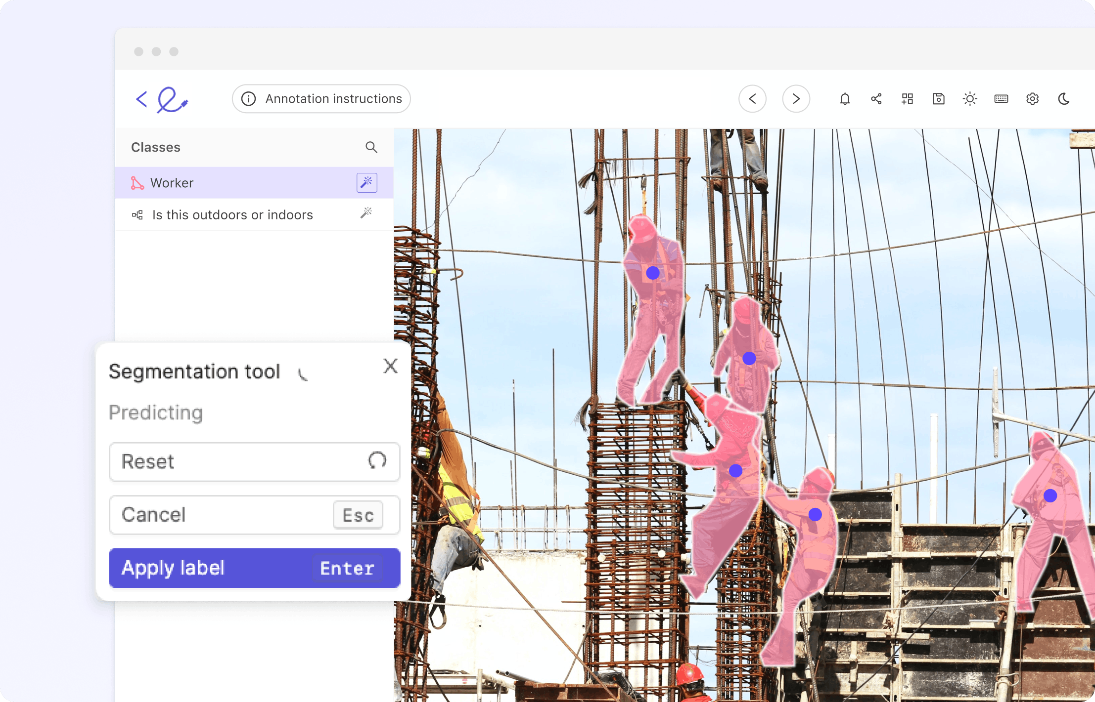
Computer vision is having its ChatGPT moment with the release of the Segment Anything Model (SAM) by Meta last week. Trained over 11 billion segmentation masks, SAM is a foundation model for predictive AI use cases rather than generative AI. While it has shown an incredible amount of flexibility in its ability to segment over wide-ranging image modalities and problem spaces, it was released without “fine-tuning” functionality. This tutorial will outline some of the key steps to fine-tune SAM using the mask decoder, particularly describing which functions from SAM to use to pre/post-process the data so that it's in good shape for fine-tuning. {{Training_data_CTA::Supercharge your annotations by fine-tuning SAM for your use case}} What is the Segment Anything Model (SAM)? The Segment Anything Model (SAM) is a segmentation model developed by Meta AI. It is considered the first foundational model for Computer Vision. SAM was trained on a huge corpus of data containing millions of images and billions of masks, making it extremely powerful. As its name suggests, SAM is able to produce accurate segmentation masks for a wide variety of images. SAM’s design allows it to take human prompts into account, making it particularly powerful for Human In The Loop annotation. These prompts can be multi-modal: they can be points on the area to be segmented, a bounding box around the object to be segmented, or a text prompt about what should be segmented. The model is structured into 3 components: an image encoder, a prompt encoder, and a mask decoder. Source The image encoder generates an embedding for the image being segmented, whilst the prompt encoder generates an embedding for the prompts. The image encoder is a particularly large component of the model. This is in contrast to the lightweight mask decoder, which predicts segmentation masks based on the embeddings. Meta AI has made the weights and biases of the model trained on the Segment Anything 1 Billion Mask (SA-1B) dataset available as a model checkpoint. {{light_callout_start}} Learn more about how Segment Anything works in our explainer blog post Segment Anything Model (SAM) Explained. {{light_callout_end}} What is Model Fine-Tuning? Publicly available state-of-the-art models have a custom architecture and are typically supplied with pre-trained model weights. If these architectures were supplied without weights then the models would need to be trained from scratch by the users, who would need to use massive datasets to obtain state-of-the-art performance. Model fine-tuning is the process of taking a pre-trained model (architecture+weights) and showing it data for a particular use case. This will typically be data that the model hasn’t seen before, or that is underrepresented in its original training dataset. The difference between fine-tuning the model and starting from scratch is the starting value of the weights and biases. If we were training from scratch, these would be randomly initialized according to some strategy. In such a starting configuration, the model would ‘know nothing’ of the task at hand and perform poorly. By using pre-existing weights and biases as a starting point we can ‘fine tune’ the weights and biases so that our model works better on our custom dataset. For example, the information learned to recognize cats (edge detection, counting paws) will be useful for recognizing dogs. Why Would I Fine-Tune a Model? The purpose of fine-tuning a model is to obtain higher performance on data that the pre-trained model has not seen before. For example, an image segmentation model trained on a broad corpus of data gathered from phone cameras will have mostly seen images from a horizontal perspective. If we tried to use this model for satellite imagery taken from a vertical perspective, it may not perform as well. If we were trying to segment rooftops, the model may not yield the best results. The pre-training is useful because the model will have learned how to segment objects in general, so we want to take advantage of this starting point to build a model that can accurately segment rooftops. Furthermore, it is likely that our custom dataset would not have millions of examples, so we want to fine-tune instead of training the model from scratch. Fine tuning is desirable so that we can obtain better performance on our specific use case, without having to incur the computational cost of training a model from scratch. How to Fine-Tune Segment Anything Model [With Code] Background & Architecture We gave an overview of the SAM architecture in the introduction section. The image encoder has a complex architecture with many parameters. In order to fine-tune the model, it makes sense for us to focus on the mask decoder which is lightweight and therefore easier, faster, and more memory efficient to fine-tune. In order to fine-tune SAM, we need to extract the underlying pieces of its architecture (image and prompt encoders, mask decoder). We cannot use SamPredictor.predict (link) for two reasons: We want to fine-tune only the mask decoder This function calls SamPredictor.predict_torch which has the @torch.no_grad() decorator (link), which prevents us from computing gradients Thus, we need to examine the SamPredictor.predict function and call the appropriate functions with gradient calculation enabled on the part we want to fine-tune (the mask decoder). Doing this is also a good way to learn more about how SAM works. Creating a Custom Dataset We need three things to fine-tune our model: Images on which to draw segmentations Segmentation ground truth masks Prompts to feed into the model We chose the stamp verification dataset (link) since it has data that SAM may not have seen in its training (i.e., stamps on documents). We can verify that it performs well, but not perfectly, on this dataset by running inference with the pre-trained weights. The ground truth masks are also extremely precise, which will allow us to calculate accurate losses. Finally, this dataset contains bounding boxes around the segmentation masks, which we can use as prompts to SAM. An example image is shown below. These bounding boxes align well with the workflow that a human annotator would go through when looking to generate segmentations. Input Data Preprocessing We need to preprocess the scans from numpy arrays to pytorch tensors. To do this, we can follow what happens inside SamPredictor.set_image (link) and SamPredictor.set_torch_image (link) which preprocesses the image. First, we can use utils.transform.ResizeLongestSide to resize the image, as this is the transformer used inside the predictor (link). We can then convert the image to a pytorch tensor and use the SAM preprocess method (link) to finish preprocessing. Training Setup We download the model checkpoint for the vit_b model and load them in: sam_model = sam_model_registry['vit_b'](checkpoint='sam_vit_b_01ec64.pth') We can set up an Adam optimizer with defaults and specify that the parameters to tune are those of the mask decoder: optimizer = torch.optim.Adam(sam_model.mask_decoder.parameters()) At the same time, we can set up our loss function, for example Mean Squared Error loss_fn = torch.nn.MSELoss() Training Loop In the main training loop, we will be iterating through our data items, generating masks, and comparing them to our ground truth masks so that we can optimize the model parameters based on the loss function. In this example, we used a GPU for training since it is much faster than using a CPU. It is important to use .to(device) on the appropriate tensors to make sure that we don’t have certain tensors on the CPU and others on the GPU. We want to embed images by wrapping the encoder in the torch.no_grad() context manager, since otherwise we will have memory issues, along with the fact that we are not looking to fine-tune the image encoder. with torch.no_grad(): image_embedding = sam_model.image_encoder(input_image) We can also generate the prompt embeddings within the no_grad context manager. We use our bounding box coordinates, converted to pytorch tensors. with torch.no_grad(): sparse_embeddings, dense_embeddings = sam_model.prompt_encoder( points=None, boxes=box_torch, masks=None, ) Finally, we can generate the masks. Note that here we are in single mask generation mode (in contrast to the 3 masks that are normally output). low_res_masks, iou_predictions = sam_model.mask_decoder( image_embeddings=image_embedding, image_pe=sam_model.prompt_encoder.get_dense_pe(), sparse_prompt_embeddings=sparse_embeddings, dense_prompt_embeddings=dense_embeddings, multimask_output=False, ) The final step here is to upscale the masks back to the original image size since they are low resolution. We can use Sam.postprocess_masks to achieve this. We will also want to generate binary masks from the predicted masks so that we can compare these to our ground truths. It is important to use torch functionals in order to not break backpropagation. upscaled_masks = sam_model.postprocess_masks(low_res_masks, input_size, original_image_size).to(device) from torch.nn.functional import threshold, normalize binary_mask = normalize(threshold(upscaled_masks, 0.0, 0)).to(device) Finally, we can calculate the loss and run an optimization step: loss = loss_fn(binary_mask, gt_binary_mask) optimizer.zero_grad() loss.backward() optimizer.step() By repeating this over a number of epochs and batches we can fine-tune the SAM decoder. Saving Checkpoints and Starting a Model from it Once we are done with training and satisfied with the performance uplift, we can save the state dict of the tuned model using: torch.save(model.state_dict(), PATH) We can then load this state dict when we want to perform inference on data that is similar to the data we used to fine-tune the model. {{light_callout_start}} You can find the Colab Notebook with all the code you need to fine-tune SAM here. Keep reading if you want a fully working solution out of the box! {{light_callout_end}} Fine-Tuning for Downstream Applications While SAM does not currently offer fine-tuning out of the box, we are building a custom fine-tuner integrated with the Encord platform. As shown in this post, we fine-tune the decoder in order to achieve this. This is available as an out-of-the-box one-click procedure in the web app, where the hyperparameters are automatically set. Original vanilla SAM mask: Mask generated by fine-tuned version of the model: We can see that this mask is tighter than the original mask. This was the result of fine-tuning on a small subset of images from the stamp verification dataset, and then running the tuned model on a previously unseen example. With further training and more examples, we could obtain even better results. Conclusion That's all, folks! You have now learned how to fine-tune the Segment Anything Model (SAM). If you're looking to fine-tune SAM out of the box, you might also be interested to learn that we have recently released the Segment Anything Model in Encord, allowing you to fine-tune the model without writing any code. {{SAM_CTA}}
Read more
Phi-3 is a family of open artificial intelligence models developed by Microsoft. These models have quickly gained popularity for being the most capable and cost-effective small language models (SLMs) available. The Phi-3 models, including Phi-3-mini, are cost-effective and outperform models of the same size and even the next size across various benchmarks of language, reasoning, coding, and math. Let’s discuss how these models in detail. What are Small Language Models (SLM)? Small Language Models (SLMs) refer to scaled-down versions of large language models (LLMs) like OpenAI’s GPT, Meta’s LLama-3, Mistral 7B, etc. These models are designed to be more lightweight and efficient both in terms of computational resources for training and inference for simpler tasks and in their memory footprint. The “small” in SLMs refers to the number of parameters that the model has. These models are typically trained on a large corpus of high-quality data and learn to predict the next work in a sentence, which allows them to generate coherent and contextually relevant sentences. These lightweight AI models are typically used in scenarios where computational resources are limited or where real-time inference is necessary. They sacrifice some performance and capabilities compared to their larger counterparts but still provide valuable language understanding and generation capabilities. SLMs find applications in various fields such as mobile devices, IoT devices, edge computing, and scenarios that have low-latency interactions. They allow for more widespread deployment of natural language processing capabilities in resource-constrained environments. Microsoft's Phi-3 is a prime example of an SLM that pushes the boundaries of what's possible with these models, offering superior performance across various benchmarks while being cost-effective. Phi-3: Introducing Microsoft’s SLM Tech giant Microsoft launches Phi-3, a Small Language Model (SLM) designed to deliver great performance while remaining lightweight enough to run on resource-constrained devices like smartphones. With an impressive 3.8 billion parameters, Phi-3 represents a significant milestone in compact language modeling technology. Prioritizing techniques in dataset curation and model architecture, Phi-3 achieves competitive performance comparable to much larger models like Mixtral 8x7B and GPT-3.5. Performance Evaluation Phi-3's performance is assessed through rigorous evaluation against academic benchmarks and internal testing. Despite its smaller size, Phi-3 demonstrates impressive results, achieving 69% on the MMLU benchmark and 8.38 on the MT-bench metric. Phi-3 Technical Report: A Highly Capable Language Model Locally on Your Phone When comparing the performance of Phi-3 with GPT-3.5, a Large Language Model (LLM), it's important to consider the tasks at hand. For many language, reasoning, coding, and math benchmarks, Phi-3 models have been shown to outperform models of the same size and those of the next size up, including GPT-3.5. Phi-3 Architecture Phi-3 is a transformer decoder architecture with a default context length of 4K, ensuring efficient processing of input data while maintaining context awareness. Phi-3 also offers a long context version, Phi-3-mini-128K, extending context length to 128K for handling tasks requiring broader context comprehension. With 32 heads and 32 layers, Phi-3 balances model complexity with computational efficiency, making it suitable for deployment on mobile devices. Microsoft Phi-3: Model Training Process The model training process for Microsoft's Phi-3 has a comprehensive approach: High-Quality Data Training Phi-3 is trained using high-quality data curated from various sources, including heavily filtered web data and synthetic data. This meticulous data selection process ensures that the model receives diverse and informative input to enhance its language understanding and reasoning capabilities. Extensive Post-training Post-training procedures play a crucial role in refining Phi-3's performance and ensuring its adaptability to diverse tasks and scenarios. Through extensive post-training techniques, including supervised fine-tuning and direct preference optimization, Phi-3 undergoes iterative improvement to enhance its proficiency in tasks such as math, coding, reasoning, and conversation. Reinforcement Learning from Human Feedback (RLHF) Microsoft incorporates reinforcement learning from human feedback (RLHF) into Phi-3's training regime. This mechanism allows the model to learn from human interactions, adapting its responses based on real-world feedback. RLHF enables Phi-3 to continuously refine its language generation capabilities, ensuring more contextually appropriate and accurate responses over time. If you are looking to integrate RLHF into your ML pipeline, read the blog Top Tools for RLHF to find the right tools for your project. Automated Testing Phi-3's training process includes rigorous automated testing procedures to assess model performance and identify potential areas for improvement. Automated testing frameworks enable efficient evaluation of Phi-3's functionality across various linguistic tasks and domains, facilitating ongoing refinement and optimization. Manual Red-teaming In addition to automated testing, Phi-3 undergoes manual red-teaming, wherein human evaluators systematically analyze model behavior and performance. This manual assessment process provides valuable insights into Phi-3's strengths and weaknesses, guiding further training iterations and post-training adjustments to enhance overall model quality and reliability. Advantages of Phi-3: SLM Vs. LLM Small Language Model (SLM), offers several distinct advantages over traditional Large Language Models (LLMs), highlighting its suitability for a variety of applications and deployment scenarios. Resource Efficiency: SLMs like Phi-3 are designed to be more resource-efficient compared to LLMs. With its compact size and optimized architecture, Phi-3 consumes fewer computational resources during both training and inference, making it ideal for deployment on resource-constrained devices such as smartphones and IoT devices. Size and Flexibility: Phi-3-mini, a 3.8B language model, is available in two context-length variants—4K and 128K tokens1. It is the first model in its class to support a context window of up to 128K tokens, with little impact on quality. Instruction-tuned: Phi-3 models are instruction-tuned, meaning that they’re trained to follow different types of instructions reflecting how people normally communicate. Scalability: SLMs like Phi-3 offer greater scalability compared to LLMs. Their reduced computational overhead allows for easier scaling across distributed systems and cloud environments, enabling seamless integration into large-scale applications with high throughput requirements. Optimized for Various Platforms: Phi-3 models have been optimized for ONNX Runtime with support for Windows DirectML along with cross-platform support across GPU, CPU, and even mobile hardware. While LLMs will still be the gold standard for solving many types of complex tasks, SLMs like Phi-3 offer many of the same capabilities found in LLMs but are smaller in size and are trained on smaller amounts of data. For more information about the Phi-3 models, read the technical report Phi-3 Technical Report: A Highly Capable Language Model Locally on Your Phone. Quality Vs. Model Size Comparison In the trade-off between model size and performance quality, Phi-3 claims remarkable efficiency and effectiveness compared to larger models. Performance Parity Despite its smaller size, Phi-3 achieves performance parity with larger LLMs such as Mixtral 8x7B and GPT-3.5. Through innovative training methodologies and dataset curation, Phi-3 delivers competitive results on benchmark tests and internal evaluations, demonstrating its ability to rival larger models in terms of language understanding and generation capabilities. Optimized Quality Phi-3 prioritizes dataset quality optimization within its constrained parameter space, leveraging advanced training techniques and data selection strategies to maximize performance. By focusing on the quality of data and training processes, Phi-3 achieves impressive results that are comparable to, if not surpass, those of larger LLMs. Efficient Utilization Phi-3 shows efficient utilization of model parameters, demonstrating that superior performance can be achieved without exponentially increasing model size. By striking a balance between model complexity and resource efficiency, Phi-3 sets a new standard for small-scale language modeling, offering a compelling alternative to larger, more computationally intensive models. Quality of Phi-3 models’s performance on MMLU benchmark compared to other models of similar size Client Success Case Study Organizations like ITC, a leading business in India, are already using Phi-3 models to drive efficiency in their solutions. ITC's collaboration with Microsoft on the Krishi Mitra copilot, a farmer-facing app, showcases the practical impact of Phi-3 in agriculture. By integrating fine-tuned versions of Phi-3, ITC aims to improve efficiency while maintaining accuracy, ultimately enhancing the value proposition of their farmer-facing application. For more information, read the blog Generative AI in Azure Data Manager for Agriculture. Limitations of Phi-3 The limitations of Phi-3, despite its impressive capabilities, are primarily from its smaller size compared to larger Language Models (LLMs): Limited Factual Knowledge Due to its limited parameter space, Phi-3-mini may struggle with tasks that require extensive factual knowledge, as evidenced by lower performance on benchmarks like TriviaQA. The model's inability to store vast amounts of factual information poses a challenge for tasks reliant on deep factual understanding. Language Restriction Phi-3-mini primarily operates within the English language domain, which restricts its applicability in multilingual contexts. While efforts are underway to explore multilingual capabilities, such as with Phi-3-small and the inclusion of more multilingual data, extending language support remains an ongoing challenge. Dependency on External Resources To compensate for its capacity limitations, Phi-3-mini may rely on external resources, such as search engines, to augment its knowledge base for certain tasks. While this approach can alleviate some constraints, it introduces dependencies and may not always guarantee optimal performance. Challenges in Responsible AI (RAI) Like many LLMs, Phi-3 faces challenges related to responsible AI practices, including factual inaccuracies, biases, inappropriate content generation, and safety concerns. Despite diligent efforts in data curation, post-training refinement, and red-teaming, these challenges persist and require ongoing attention and mitigation strategies. For more information on Microsoft’s responsible AI practices, read Microsoft Responsible AI Standard, v2. Phi-3 Availability The first model in this family, Phi-3-mini, a 3.8B language model, is now available. It is available in two context-length variants—4K and 128K tokens. The Phi-3-mini is available on Microsoft Azure AI Model Catalog, Hugging Face, and Ollama. It has been optimized for ONNX Runtime with support for Windows DirectML along with cross-platform support across graphics processing unit (GPU), CPU, and even mobile hardware. In the coming weeks, additional models will be added to the Phi-3 family to offer customers even more flexibility across the quality-cost curve Phi-3-small (7B) and Phi-3-medium (14B) will be available in the Azure AI model catalog, and other model families shortly. It will also be available as an NVIDIA NIM microservice with a standard API interface that can be deployed anywhere. Phi-3: Key Takeaways Microsoft's Phi-3 models are small language models (SLMs) designed for efficiency and performance, boasting 3.8 billion parameters and competitive results compared to larger models. Phi-3 utilizes high-quality curated data and advanced post-training techniques, including reinforcement learning from human feedback (RLHF), to refine its performance. Its transformer decoder architecture ensures efficiency and context awareness. Phi-3 offers resource efficiency, scalability, and flexibility, making it suitable for deployment on resource-constrained devices. Despite its smaller size, it achieves performance parity with larger models through dataset quality optimization and efficient parameter utilization. While Phi-3 demonstrates impressive capabilities, limitations include limited factual knowledge and language support. It is currently available in its first model, Phi-3-mini, with plans for additional models to be added, offering more options across the quality-cost curve.
April 25
8 min
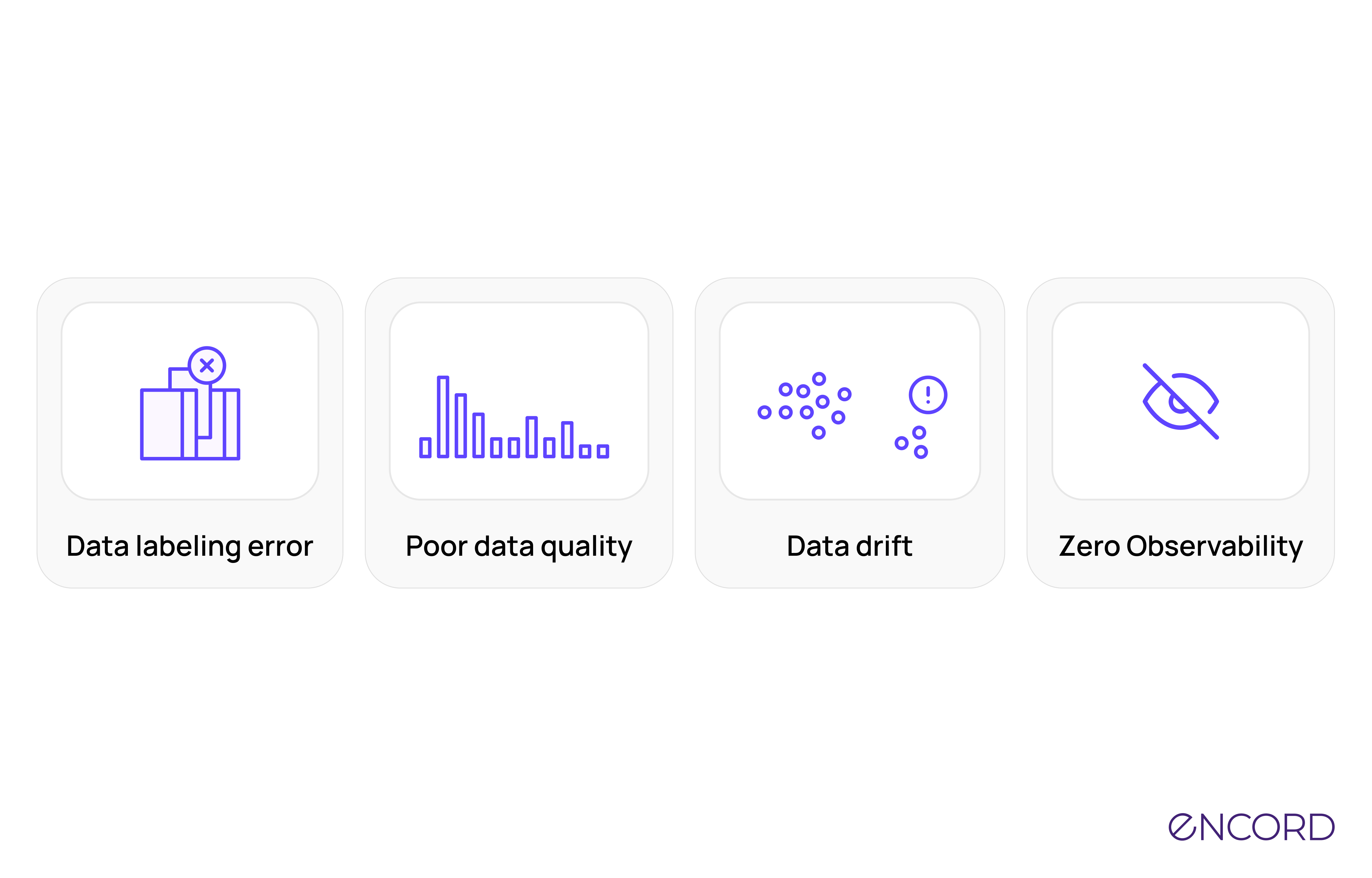
Here’s a scenario you’ve likely encountered: You spent months building your model, increased your F1 score above 90%, convinced all stakeholders to launch it, and... poof! As soon as your model sees real-world data, its performance drops below what you expected. This is a common production machine learning (ML) problem for many teams—not just yours. It can also be a very frustrating experience for computer vision (CV) engineers, ML teams, and data scientists. There are many potential factors behind these. Problems could stem from the quality of the production data, the design of the production pipelines, the model itself, or operational hurdles the system faces in production. In this article, you will learn the four (4) reasons why computer vision models fail in production and thoroughly examine the ML lifecycle stages where they occur. These reasons show you the most common production CV and data science problems. Knowing their causes may help you prevent, mitigate, or fix them. You’ll also see the various strategies for addressing these problems at each step. Let’s jump right into it! Why do Models Fail in Production? The ML lifecycle governs how ML models are developed and shipped; it involves sourcing data, data exploration and preparation (data cleaning and EDA), model training, and model deployment, where users can consume the model predictions. These processes are interdependent, as an error in one stage could affect the corresponding stages, resulting in a model that doesn’t perform well—or completely fails—in production. Organizations develop machine learning (ML) and artificial intelligence (AI) models to add value to their businesses. When errors occur at any ML development stage, they can lead to production models failing, costing businesses capital, human resources, and opportunities to satisfy customer expectations. Consider the implications of poorly labeling data for a CV model after data collection. Or the model has an inherent bias—it could invariably affect results in a production environment. It is noteworthy that the problem can start when businesses do not have precise reasons or objectives for developing and deploying machine learning models, which can cripple the process before it begins. Assuming the organization has passed all stages and deployed its model, the errors we often see that lead to models failing in production include: Mislabeling data, which can train models on incorrect information. ML engineers and CV teams that prioritize data quality only at later stages rather than as a foundational practice. Ignoring the drift in data distribution over time can make models outdated or irrelevant. Implementing minimal or no validation (quality assurance) steps risks unnoticed errors progressing to production. Viewing model deployment as the final goal, neglecting necessary ongoing monitoring and adjustments. Let’s look deeper at these errors and why they are the top reasons we see production models fail. Reason #1: Data Labeling Errors Data labeling is the foundation for training machine learning models, particularly supervised learning, where models learn patterns directly from labeled data. This involves humans or AI systems assigning informative labels to raw data—whether it be images, videos, or DICOM—to provide context that enables models to learn. AI algorithms also synthesize labeled data. Check out our guide on synthetic data and why it is useful. Despite its importance, data labeling is prone to errors, primarily because it often relies on human annotators. These errors can compromise a model's accuracy by teaching it incorrect patterns. Consider a scenario in a computer vision project to identify objects in images from data sources. Even a small percentage of mislabeled images can lead the model to associate incorrect features with an object. This could mean the model makes wrong predictions in production. Potential Solution: Automated Labeling Error Detection A potential solution is adopting tools and frameworks that automatically detect labeling errors. These tools analyze labeling patterns to identify outliers or inconsistent labels, helping annotators revise and refine the data. An example is Encord Active. Encord Active is one of three products in the Encord platform (the others are Annotate and Index) that includes features to find failure modes in your data, labels, and model predictions. A common data labeling issue is the border closeness of the annotations. Training data with many border-proximate annotations can lead to poor model generalization. If a model is frequently exposed to partially visible objects during training, it might not perform well when presented with fully visible objects in a deployment scenario. This can affect the model's accuracy and reliability in production. Let’s see how Encord Active can help you, for instance, identify border-proximate annotations. Step 1: Select your Project. Step 2: Under the “Explorer” dashboard, find the “Labels” tab. Encord Active automatically finds patterns in the data and labels to surface potential issues with the label. Step 3: On the right pane, click on one of the issues EA found to filter your data and labels by it. In this case, “Border Closeness”; click on it. “Relative Area.” - Identifies annotations that are too close to image borders. Images with a Border Proximity score of 1 are flagged as too close to the border. Step 4: Select one of the images to inspect and validate the issue. Here’s a GIF with the steps: You will notice that EA also shows you the model’s predictions alongside the annotations, so you can visually inspect the annotation issue and resulting prediction. Step 5: Visually inspect the top images EA flags and use the Collections feature to curate them. There are a few approaches you could take after creating the Collections: Exclude the images that are border-proximate from the training data if the complete structure of the object is crucial for your application. This prevents the model from learning from incomplete data, which could lead to inaccuracies in object detection. Send the Collection to annotators for review. Recommended Read: 5 Ways to Improve the Quality of Labeled Data. Reason #2: Poor Data Quality The foundation of any ML model's success lies in the quality of the data it's trained on. High-quality data is characterized by its accuracy, completeness, timeliness, and relevance to the business problem ("fit for purpose"). Several common issues can compromise data quality: Duplicate Images: They can artificially increase the frequency of particular features or patterns in the training data. This gives the model a false impression of these features' importance, causing overfitting. Noise in Images: Blur, distortion, poor lighting, or irrelevant background objects can mask important image features, hindering the model's ability to learn and recognize relevant patterns. Unrepresentative Data: When the training dataset doesn't accurately reflect the diversity of real-world scenarios, the model can develop biases. For example, a facial recognition system trained mainly on images of people with lighter skin tones may perform poorly on individuals with darker skin tones. Limited Data Variation: A model trained on insufficiently diverse data (including duplicates and near-duplicates) will struggle to adapt to new or slightly different images in production. For example, if a self-driving car system is trained on images taken in sunny weather, it might fail in rainy or snowy conditions. Potential Solution: Data Curation One way to tackle poor data quality, especially after collection, is to curate good quality data. Here is how to use Encord Active to automatically detect and classify duplicates in your set. Curate Duplicate Images Your testing and validation sets might contain duplicate training images that inflate the performance metrics. This makes the model appear better than it is, which could lead to false confidence about its real-world capabilities. Step 1: Navigate to the Explorer dashboard → Data tab On the right-hand pane, you will notice Encord Active has automatically detected common data quality issues based on the metrics it computed from the data. See an overview of the issues EA can detect on this documentation page. Step 2: Under the issues found, click on Duplicates to see the images EA flags as duplicates and near-duplicates with uniqueness scores of 0.0 to 0.00001. There are two steps you could take to solve this issue: Carefully remove duplicates, especially when dealing with imbalanced datasets, to avoid skewing the class distribution further. If duplicates cannot be fully removed (e.g., to maintain the original distribution of rare cases), use data augmentation techniques to introduce variations within the set of duplicates themselves. This can help mitigate some of the overfitting effects. Step 3: Under the Data tab, curate duplicates you want to remove or use augmentation techniques to improve by selecting them. Click Add to a Collection → Name the collection ‘Duplicates’ and add a description. See the complete steps: Once the duplicates are in the Collection, you can use the tag to filter them out of your training or validation data. If relevant, you can also create a new dataset to apply the data augmentation techniques. Other solutions could include: Implement Robust Data Validation Checks: Use automated tools that continuously validate data accuracy, consistency, and completeness at the entry point (ingestion) and throughout the data pipeline. Adopt a Centralized Data Management Platform: A unified view of data across sources (e.g., data lakes) can help identify discrepancies early and simplify access for CV engineers (or DataOps teams) to maintain data integrity. See Also: Improving Data Quality Using End-to-End Data Pre-Processing Techniques in Encord Active. Reason #3: Data Drift Data drift occurs when the statistical properties of the real-world images a model encounters in production change over time, diverging from the samples it was trained on. Drift can happen due to various factors, including: Concept Drift: The underlying relationships between features and the target variable change. For example, imagine a model trained to detect spam emails. The features that characterize spam (certain keywords, sender domains) can evolve over time. Covariate Shift: The input feature distribution changes while the relationship to the target variable remains unchanged. For instance, a self-driving car vision system trained in summer might see a different distribution of images (snowy roads, different leaf colors) in winter. Prior Probability Shift: The overall frequency of different classes changes. For example, a medical image classification model trained for a certain rare disease may encounter it more frequently as its prevalence changes in the population. If you want to dig deeper into the causes of drifts, check out the “Data Distribution Shifts and Monitoring” article. Potential Solution: Monitoring Data Drift There are two steps you could take to address data drift: Use tools that monitor the model's performance and the input data distribution. Look for shifts in metrics and statistical properties over time. Collect new data representing current conditions and retrain the model at appropriate intervals. This can be done regularly or triggered by alerts when significant drift is detected. You can achieve both within Encord: Step 1: Create the Dataset on Annotate to log your input data for training or production. If your data is on a cloud platform, check out one of the data integrations to see if it works with your stack. Step 2: Create an Ontology to define the structure of the dataset. Step 3: Create an Annotate Project based on your dataset and the ontology. Ensure the project also includes Workflows because some features in Encord Active only support projects that include workflows. Step 4: Import your Annotate Project to Active. This will allow you to import the data, ground truth, and any custom metrics to evaluate your data quality. See how it’s done in the video tutorial on the documentation. Step 5: Select the Project → Import your Model Predictions. There are two steps to inspect the issues with the input data: Use the analytics view to get a statistical summary of the data. Use the issues found by Encord Active to manually inspect where your model is struggling. Step 6: On the Explorer dashboard → Data tab → Analytics View. Step 7: Under the Metric Distribution chart, select a quality metric to assess the distribution of your input data on. In this example, “Diversity" applies algorithms to rank images from easy to hard samples to annotate. Easy samples have lower scores, while hard samples have higher scores. Step 8: On the right-hand pane, click on Dark. Navigate back to Grid View → Click on one of the images to inspect the ground truth (if available) vs. model predictions. Observe that the poor lightning could have caused the model to misidentify the toy bear as a person. (Of course, other reasons, such as class imbalance, could cause the model to misclassify the object.) You can inspect the class balance on the Analytics View → Class Distribution chart. Nice! Recommended Read: How to Detect Data Drift on Datasets. There are other ways to manage data drift, including the following approaches: Adaptive Learning: Consider online learning techniques where the model continuously updates itself based on new data without full retraining. Note that this is still an active area of research with challenges in computer vision. Domain Adaptation: If collecting substantial amounts of labeled data from the new environment is not feasible, use domain adaptation techniques to bridge the gap between the old and new domains. Recommended Read:A Practical Guide to Active Learning for Computer Vision. Reason #4: Thinking Deployment is the Final Step (No Observability) Many teams mistakenly treat deployment as the finish line, which is one reason machine learning projects fail in production. However, it's crucial to remember that this is simply one stage in a continuous cycle. Models in production often degrade over time due to factors such as data drift (changes in input data distribution) or model drift (changes in the underlying relationships the model was trained on). Neglecting post-deployment maintenance invites model staleness and eventual failure. This is where MLOps (Machine Learning Operations) becomes essential. MLOps provides practices and technologies to monitor, maintain, and govern ML systems in production. Potential Solution: Machine Learning Operations (MLOps) The core principle of MLOps is ensuring your model provides continuous business value while in production. How teams operationalize ML varies, but some key practices include: Model Monitoring: Implement monitoring tools to track performance metrics (accuracy, precision, etc.) and automatically alert you to degradation. Consider a feedback loop to trigger retraining processes where necessary, either for real-time or batch deployment. Logging: Even if full MLOps tools aren't initially feasible, start by logging model predictions and comparing them against ground truth, like we showed above with Encord. This offers early detection of potential issues. Management and Governance: Establish reproducible ML pipelines for continuous training (CT) and automate model deployment. From the start, consider regulatory compliance issues in your industry. Recommended Read:Model Drift: Best Practices to Improve ML Model Performance. Key Takeaways: 4 Reasons Computer Vision Models Fail in Production Remember that model deployment is not the last step. Do not waste time on a model only to have it fail a few days, weeks, or months later. ML systems differ across teams and organizations, but most failures are common. If you study your ML system, you’ll likely see that some of the reasons your model fails in production are similar to those listed in this article: 1. Data labelling errors 2. Poor data quality 3. Data drift in production 4. Thinking deployment is the final step The goal is for you to understand these failures and learn the best practices to solve or avoid them. You’d also realize that while most failure modes are data-centric, others are technology-related and involve team practices, culture, and available resources.
April 24
8 min
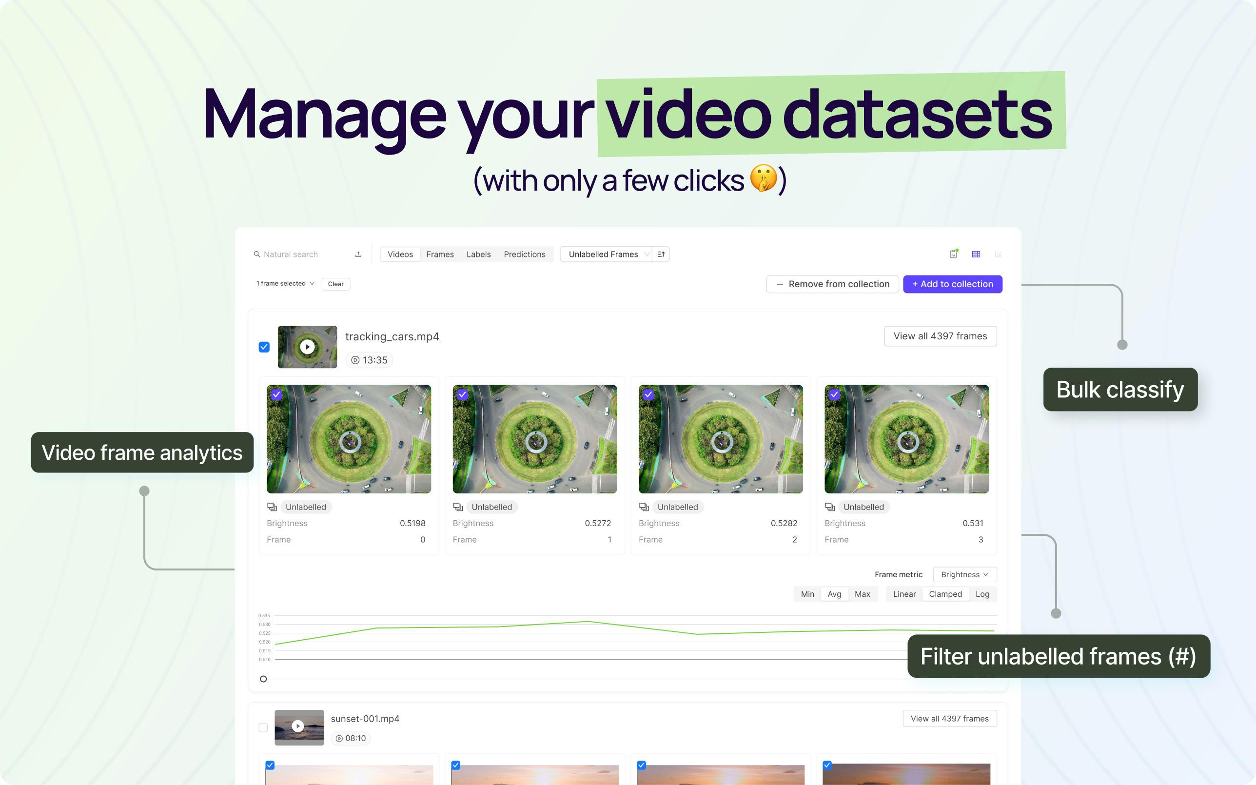
At Encord we continually look for ways to enable our customers to bring their models to market faster. Today, we’re announcing the launch of Video Data Management within the Encord Platform, providing an entirely new way to interact with video data. Gone are the days of searching frame by frame for the relevant clip. Now filter and search across your entire dataset of videos with just a few clicks. What is Advanced Video Curation? In our new video explorer page users can search, filter, and sort entire datasets of videos. Video-level metrics, calculated by taking an average from the frames of a video, allow the user to curate videos based on a range of characteristics, including average brightness, average sharpness, the number of labeled frames, and many more. Users can also curate within individual videos with the new video frame analytics timelines, enabling a temporal view over the entire video. We're thrilled that Video Data Curation in the Encord platform is the first and only platform available to search, query, and curate relevant video clips as part of your data workflows. Support within Encord This is now available for all Encord Active customers. Please see our documentation for more information on activating this tool. For any questions on how to get access to video curation please contact sales@encord.com.
April 24
2 min
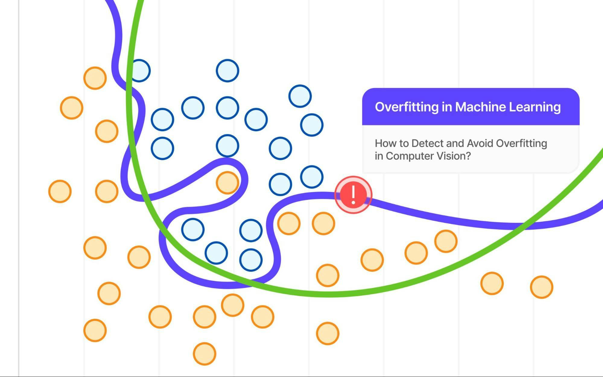
What is overfitting in computer vision? Overfitting is a significant issue in computer vision where model learns the training data too well, including noise and irrelevant details. This leads to poor performance on new unseen data even if the model performs too well on training data. Overfitting occurs when the model memorizes specific patterns in the training images instead of learning general features. Overfit models have extremely high accuracy on the training data but much lower accuracy on testing data, failing to generalize well. Complex models with many parameters are more prone to overfitting, especially with limited training data. In this blog, we will learn about What is the difference between overfitting and underfitting? How to find out if the model is overfitting? What to do if the model is overfitting? and how to use tools like Encord Active to detect and avoid overfitting. Overfitting Vs Underfitting: Key Differences Performance on training data: Overfitting leads to very high training accuracy while underfitting results in low training accuracy. Performance on test/validation data: Overfitting causes poor performance on unseen data, while underfitting also performs poorly on test/validation data. Model complexity: Overfitting is caused by excessive model complexity while underfitting is due to oversimplified models. Generalization: Overfitting models fail to generalize well, while underfit models cannot capture the necessary patterns for generalization. Bias-variance trade-off: Overfitting has high variance and low bias, while underfitting has high bias and low variance. Overfitting and Underfitting: Key Statistical Terminologies When training a machine learning model you are always trying to strike a balance between capturing the underlying patterns in the data while avoiding overfitting or underfitting. Here is a brief overview of the key statistical concepts which are important to understand for us to improve model performance and generalization. Data Leakage Data leakage occurs when information from outside the training data is used to create the model. This can lead to a situation where the model performs exceptionally well on training data but poorly on unseen data. This can happen when data preprocessing steps, such as feature selection or data imputation, are performed using information from the entire dataset, including the test set. Bias Bias refers to the error introduced by approximating a real-world problem with a simplified model. A high bias model needs to be more accurate in order to capture the underlying patterns in the data, which leads to underfitting. Addressing bias involves increasing model complexity or using more informative features. For more information on how to address bias, read the blog How To Mitigate Bias in Machine Learning Models. Variance Variance is a measure of how much the model’s predictions fluctuate for different training datasets. A high variance model is overly complex and sensitive to small fluctuations in the training data and captures noise in the training dataset. This leads to overfitting and the machine learning model performs poorly on unseen data. Bias-variance tradeoff The bias-variance tradeoff illustrates the relationship between bias and variance in the model performance. Ideally, you would want to choose a model that both accurately captures the patterns in the training data, but also generalize well to unseen data. Unfortunately, it is typically impossible to do both simultaneously. High-variance learning methods may be able to represent their training dataset well but are at risk of overfitting to noisy or unrepresented training data. In contrast, algorithms with a high bias typically produce simpler models that don’t tend to overfit but may underfit their training data, failing to capture the patterns in the dataset. Bias and variance are one of the fundamental concepts of machine learning. If you want to understand better with visualization, watch the video below. Bootstrap Bootstrapping is a statistical technique that involves resampling the original dataset with replacement to create multiple subsets or bootstrap samples. These bootstrap samples are then used to train multiple models, allowing for the estimation of model performance metrics, such as bias and variance, as well as confidence intervals for the model's predictions. K-Fold Cross-Validation K-Fold Cross-Validation is another resampling technique used to estimate a model's performance and generalization capability. The dataset is partitioned into K equal-sized subsets (folds). The model is trained on K-1 folds and evaluated on the remaining fold. This process is repeated K times, with each fold serving as the validation set once. The final performance metric is calculated as the average across all K iterations. LOOCV (Leave-One-Out Cross-Validation) Leave-One-Out Cross-Validation (LOOCV) is a special case of K-Fold Cross-Validation, where K is equal to the number of instances in the dataset. In LOOCV, the model is trained on all instances except one, and the remaining instance is used for validation. This process is repeated for each instance in the dataset, and the performance metric is calculated as the average across all iterations. LOOCV is computationally expensive but can provide a reliable estimate of model performance, especially for small datasets. Here is an amazing video by Josh Starmer explaining cross-validation. Watch it for more information. Assessing Model Fit Residual Analysis Residuals are the differences between the observed values and the values predicted by the model. Residual analysis involves examining the patterns and distributions of residuals to identify potential issues with the model fit. Ideally, residuals should be randomly distributed and exhibit no discernible patterns or trends. Structured patterns in the residuals may indicate that the model is missing important features or violating underlying assumptions. Goodness-of-Fit Tests Goodness-of-fit tests provide a quantitative measure of how well the model's predictions match the observed data. These tests typically involve calculating a test statistic and comparing it to a critical value or p-value to determine the significance of the deviation between the model and the data. Common goodness-of-fit tests include: Chi-squared test Kolmogorov-Smirnov test Anderson-Darling test The choice of test depends on the assumptions about the data distribution and the type of model being evaluated. Evaluation Metrics Evaluation metrics are quantitative measures that summarize the performance of a model on a specific task. Different metrics are appropriate for different types of problems, such as regression, classification, or ranking. Some commonly used evaluation metrics include: For regression problems: Mean Squared Error (MSE), Root Mean Squared Error (RMSE), R-squared (R²) For classification problems: Accuracy, Precision, Recall, F1-score, Area Under the Receiver Operating Characteristic Curve (AUROC) Diagnostic Plots Diagnostics plots, such as residual plots, quantile-quantile (Q-Q) plots, and calibration plots, can provide valuable insights into model fit. These graphical representations can help identify patterns, outliers, and deviations from the expected distributions, complementing the quantitative assessment of model fit. Causes for Overfitting in Computer Vision Here are the following causes for overfitting in computer vision: High Model Complexity Relative to Data Size One of the primary causes of overfitting is when the model's complexity is disproportionately high compared to the size of the training dataset. Deep neural networks, especially those used in computer vision tasks, often have millions or billions of parameters. If the training data is limited, the model can easily memorize the training examples, including their noise and peculiarities, rather than learning the underlying patterns that generalize well to new data. Noise Training Data Image or video datasets, particularly those curated from real-world scenarios, can contain a significant amount of noise, such as variations in lighting, occlusions, or irrelevant background clutter. If the training data is noisy, the model may learn to fit this noise instead of focusing on the relevant features. Insufficient Regularization Regularization techniques, such as L1 and L2 regularization, dropout, or early stopping, are essential for preventing overfitting in deep learning models. These techniques introduce constraints or penalties that discourage the model from learning overly complex patterns that are specific to the training data. With proper regularization, models can easily fit, especially when dealing with high-dimensional image data and deep network architectures. Data Leakage Between Training/Validation Sets Data leakage occurs when information from the test or validation set is inadvertently used during the training process. This can happen due to improper data partitioning, preprocessing steps that involve the entire dataset, or other unintentional sources of information sharing between the training and evaluation data. Even minor data leakage can lead to overly optimistic performance estimates and a failure to generalize to truly unseen data. How to Detect an Overfit Model? Here are some common techniques to detect an overfit model: Monitoring the Training and Validation/Test Error During the training process, track the model’s performance on both the training and validation/test datasets. If the training error continues to decrease while the validation/test error starts to increase or plateau, a strong indication of overfitting. An overfit model will have a significantly lower training error compared to the validation/test error. Learning Curves Plot learning curves that show the training and validation/test error as a function of the training set size. If the training error continues to decrease while the validation/test error remains high or starts to increase as more data is added, it suggests overfitting. An overfit model will have a large gap between the training and validation/test error curves. Cross-Validation Perform k-fold cross-validation on the training data to get an estimate of the model's performance on unseen data. If the cross-validation error is significantly higher than the training error, it may indicate overfitting. Regularization Apply regularization techniques, such as L1 (Lasso) or L2 (Ridge) regularization, dropout, or early stopping. If adding regularization significantly improves the model's performance on the validation/test set while slightly increasing the training error, it suggests that the original model was overfitting. Model Complexity Analysis Examine the model's complexity, such as the number of parameters or the depth of a neural network. A highly complex model with a large number of parameters or layers may be more prone to overfitting, especially when the training data is limited. Visualization For certain types of models, like decision trees or neural networks, visualizing the learned representations or decision boundaries can provide insights into overfitting. If the model has overly complex decision boundaries or representations that appear to fit the training data too closely, it may be an indication of overfitting. Ways to Avoid Overfitting in Computer Vision Data Augmentation Data augmentation techniques, such as rotation, flipping, scaling, and translation, can be applied to the training dataset to increase its diversity and variability. This helps the model learn more robust features and prevents it from overfitting to specific data points. Observe and Monitor the Class Distributions of Annotated Samples During annotation, observe class distributions in the dataset. If certain classes are underrepresented, use active learning to prioritize labeling unlabeled samples from those minority classes. Encord Active can help find similar images or objects to the underrepresented classes, allowing you to prioritize labeling them, thereby reducing data bias. Finding similar images in Encord Active. Early Stopping Early stopping is a regularization technique that involves monitoring the model's performance on a validation set during training. If the validation loss stops decreasing or starts to increase, it may indicate that the model is overfitting to the training data. In such cases, the training process can be stopped early to prevent further overfitting. Dropout Dropout is another regularization technique that randomly drops (sets to zero) a fraction of the activations in a neural network during training. This helps prevent the model from relying too heavily on any specific set of features and encourages it to learn more robust and distributed representations. L1 and L2 Regularization L1 and L2 regularization techniques add a penalty term to the loss function, which discourages the model from having large weights. This helps prevent overfitting by encouraging the model to learn simpler and more generalizable representations. Transfer Learning Transfer learning involves using a pre-trained model on a large dataset (e.g., ImageNet) as a starting point for training on a new, smaller dataset. The pre-trained model has already learned useful features, which can help prevent overfitting and improve generalization on the new task. Ensemble Methods Ensemble methods, such as bagging (e.g., random forests) and boosting (e.g., AdaBoost), combine multiple models to make predictions. These techniques can help reduce overfitting by averaging out the individual biases and errors of the component models. For more information, read the blog What is Ensemble Learning? Model Evaluation Regularly monitoring the model's performance on a held-out test set and evaluating its generalization capabilities is essential for detecting and addressing overfitting issues. Using Encord Active to Reduce Model Overfitting Encord Active is a comprehensive platform offering features to curate a dataset that can help reduce the model overfitting and evaluate the model’s performance to identify and address any potential issues. Here are a few of the ways Encord Active can be used to reduce model overfitting: Evaluating Training Data with Data and Label Quality Metrics Encord Active allows users to assess the quality of their training data with data quality metrics. It provides metrics such as missing values, data distribution, and outliers. By identifying and addressing data anomalies, practitioners can ensure that their dataset is robust and representative. Encord Active also allows you to ensure accurate and consistent labels for your training dataset. The label quality metrics, along with the label consistency checks and label distribution analysis help in finding noise or anomalies which contribute to overfitting. Evaluating Model Performance with Model Quality Metrics After training a model, it’s essential to evaluate its performance thoroughly. Encord Active provides a range of model quality metrics, including accuracy, precision, recall, F1-score, and area under the receiver operating characteristic curve (AUC-ROC). These metrics help practitioners understand how well their model generalizes to unseen data and identify the data points which contribute to overfitting. Active Learning Workflow Overfitting often occurs when models are trained on insufficient or noisy data. Encord Active incorporates active learning techniques, allowing users to iteratively select the most informative samples for labeling. By actively choosing which data points to label, practitioners can improve model performance while minimizing overfitting.
April 19
8 min
Multimodal deep learning is a recent trend in artificial intelligence (AI) that is revolutionizing how machines understand the real world using multiple data modalities, such as images, text, video, and audio. In particular, multiple machine learning frameworks are emerging that exploit visual representations to infer textual descriptions following Open AI’s introduction of the Contrastive Language-Image Pre-Training (CLIP) model. The improved models use more complex datasets to change the CLIP framework for use cases that are specific to the domain. They also have better state-of-the-art (SoTA) generalization performance than the models that came before them. This article discusses the benefits, challenges, and alternatives of Open AI CLIP to help you choose a model for your specific domain. The list below mentions the architectures covered: Pubmed CLIP PLIP SigLIP Street CLIP Fashion CLIP CLIP-Rscid BioCLIP CLIPBert Open AI CLIP Model CLIP is an open-source vision-language AI model by OpenAI trained using image and natural language data to perform zero-shot classification tasks. Users can provide textual captions and use the model to assign a relevant label to the query image. Open AI CLIP Model: Architecture and Development The training data consists of images from the internet and 32,768 text snippets assigned to each image as its label. The training task involves using natural language processing (NLP) to predict which label goes with which image by understanding visual concepts and relating them to the textual data. CLIP Architecture The model primarily uses an image and a text encoder that convert images and labels into embeddings. Optimization involves minimizing a contrastive loss function by computing similarity scores between these embeddings and associating the correct label with an image. See Also: What is Vector Similarity Search? Once trained, the user can provide an unseen image as input with multiple captions to the image and text encoders. CLIP will then predict the correct label that goes with the image. Benefits of OpenAI CLIP OpenAI CLIP has multiple benefits over traditional vision models. The list below mentions the most prominent advantages: Zero-shot Learning (ZSL): CLIP’s training approach allows it to label unseen images without requiring expensive training on new datasets. Like Generative Pre-trained Transformer - 3 (GPT-3) and GPT-4, CLIP can perform zero-shot classification tasks using natural language data with minimal training overhead. The property also helps users fine-tune CLIP more quickly to adapt to new tasks. Better Real-World Performance: CLIP demonstrates better real-world performance than traditional vision models, which only work well with benchmark datasets. Limitations of OpenAI CLIP Although CLIP is a robust framework, it has a few limitations, as highlighted below: Poor Performance on Fine-grained Tasks: CLIP needs to improve its classification performance for fine-grained tasks such as distinguishing between car models, animal species, flower types, etc. Out-of-Distribution Data: While CLIP performs well on data with distributions similar to its training set, performance drops when it encounters out-of-distribution data. The model requires more diverse image pre-training to generalize to entirely novel tasks. Inherent Social Bias: The training data used for CLIP consists of randomly curated images with labels from the internet. The approach implies the model learns intrinsic biases present in image captions as the image-text pairs do not undergo filtration. Due to these limitations, the following section will discuss a few alternatives for domain-specific tasks. Learn how to build visual search engines with CLIP and ChatGPT in our on-demand webinar. Alternatives to CLIP Since CLIP’s introduction, multiple vision-language algorithms have emerged with unique capabilities for solving problems in healthcare, fashion, retail, etc. We will discuss a few alternative models that use the CLIP framework as their base. We will also briefly mention their architecture, development approaches, performance results, and use cases. 1. PubmedCLIP PubmedCLIP is a fine-tuned version of CLIP for medical visual question-answering (MedVQA), which involves answering natural language questions about an image containing medical information. PubmedCLIP: Architecture and Development The model is pre-trained on the Radiology Objects in Context (ROCO) dataset, which consists of 80,000 samples with multiple image modalities, such as X-ray, fluoroscopy, mammography, etc. The image-text pairs come from Pubmed articles; each text snippet briefly describes the image’s content. PubmedCLIP Architecture Pre-training includes fine-tuning CLIP’s image and text encoders to minimize contrastive language and vision loss. The pretrained module, PubMedCLIP, and a Convolutional Denoising Image Autoencoder (CDAE) encode images. A question encoder converts natural language questions into embeddings and combines them with the encoded image through a bilinear attention network (BAN). The training objective is to map the embeddings with the correct answer by minimizing answer classification and image reconstruction loss using a CDAE decoder. Performance Results of PubmedCLIP The accuracy metric shows an improvement of 1% compared to CLIP on the VQA-RAD dataset, while PubMedCLIP with the vision transform ViT-32 as the backend shows an improvement of 3% on the SLAKE dataset. See Also: Introduction to Vision Transformers (ViT). PubmedCLIP: Use Case Healthcare professionals can use PubMedCLIP to interpret complex medical images for better diagnosis and patient care. 2. PLIP The Pathology Language-Image Pre-Training (PLIP) model is a CLIP-based framework trained on extensive, high-quality pathological data curated from open social media platforms such as medical Twitter. PLIP: Architecture and Development Researchers used 32 pathology hashtags according to the recommendations of the United States Canadian Academy for Pathology (USCAP) and the Pathology Hashtag Ontology project. The hashtags helped them retrieve relevant tweets containing de-identified pathology images and natural descriptions. The final dataset - OpenPath - comprises 116,504 image-text pairs from Twitter posts, 59,869 image-text pairs from the corresponding replies with the highest likes, and 32,041 additional image-text pairs from the internet and the LAION dataset. OpenPath Dataset Experts use OpenPath to fine-tune CLIP through an image preprocessing pipeline that involves image down-sampling, augmentations, and random cropping. Performance Results of PLIP PLIP achieved state-of-the-art (SoTA) performance across four benchmark datasets. On average, PLIP achieved an F1 score of 0.891, while CLIP scored 0.813. PLIP: Use Case PLIP aims to classify pathological images for multiple medical diagnostic tasks and help retrieve unique pathological cases through image or natural language search. New to medical imaging? Check out ‘Guide to Experiments for Medical Imaging in Machine Learning.’ 3. SigLip SigLip uses a more straightforward sigmoid loss function to optimize the training process instead of a softmax contrastive loss as traditionally used in CLIP. The method boosts training efficiency and allows users to scale the process when developing models using more extensive datasets. SigLip: Architecture and Development Optimizing the contrastive loss function implies maximizing the distance between non-matching image-text pairs while minimizing the distance between matching pairs. However, the method requires text-to-image and image-to-text permutations across all images and text captions. It also involves computing normalization factors to calculate a softmax loss. The approach is computationally expensive and memory-inefficient. Instead, the sigmoid loss simplifies the technique by converting the loss into a binary classification problem by assigning a positive label to matching pairs and negative labels to non-matching combinations. Efficient Loss Implementation In addition, permutations occur on multiple devices, with each device predicting positive and negative labels for each image-text pair. Later, the devices swap the text snippets to re-compute the loss with corresponding images. Performance Results of SigLip Based on the accuracy metric, the sigmoid loss outperforms the softmax loss for smaller batch sizes on the ImageNet dataset. Performance comparison Both losses deteriorate after a specific batch size, with Softmax performing slightly better at substantial batch sizes. SigLip: Use Case SigLip is suitable for training tasks involving extensive datasets. Users can fine-tune SigLip using smaller batch sizes for faster training. 4. StreetCLIP StreetCLIP is an image geolocalization algorithm that fine-tunes CLIP on geolocation data to predict the locations of particular images. The model is available on Hugging Face for further research. StreetCLIP: Architecture and Development The model improves CLIP zero-shot learning capabilities by training a generalized zero-shot learning (GZSL) classifier that classifies seen and unseen images simultaneously during the training process. StreetCLIP Architecture Fine-tuning involves generating synthetic captions for each image, specifying the city, country, and region. The training objective is to correctly predict these three labels for seen and unseen photos by optimizing a GZSL and a vision representation loss. Performance Results of StreetCLIP Compared to CLIP, StreetCLIP has better geolocation prediction accuracy. It outperforms CLIP by 0.3 to 2.4 percentage points on the IM2GPS and IM2GPS3K benchmarks. StreetCLIP: Use Case StreetCLIP is suitable for navigational purposes where users require information on weather, seasons, climate patterns, etc. It will also help intelligence agencies and journalists extract geographical information from crime scenes. 5. FashionCLIP FashionCLIP (F-CLIP) fine-tunes the CLIP model using fashion datasets consisting of apparel images and textual descriptions. The model is available on GitHub and HuggingFace. FashionCLIP: Architecture and Development The researchers trained the model on 700k image-text pairs in the Farfetch inventory dataset and evaluated it on image retrieval and classification tasks. F-CLIP Architecture The evaluation also involved testing for grounding capability. For instance, zero-shot segmentation assessed whether the model understood fashion concepts such as sleeve length, brands, textures, and colors. They also evaluated compositional understanding by creating improbable objects to see if F-CLIP generated appropriate captions. For instance, they see if F-CLIP can generate a caption—a Nike dress—when seeing a picture of a long dress with the Nike symbol. Performance Results of FashionCLIP F-CLIP outperforms CLIP on multiple benchmark datasets for multi-modal retrieval and product classification tasks. For instance, F-CLIP's F1 score for product classification is 0.71 on the F-MNIST dataset, while it is 0.66 for CLIP. FashionCLIP: Use Case Retailers can use F-CLIP to build chatbots for their e-commerce sites to help customers find relevant products based on specific text prompts. The model can also help users build image-generation applications for visualizing new product designs based on textual descriptions. 6. CLIP-RSICD CLIP-RSICD is a fine-tuned version of CLIP trained on the Remote Sensing Image Caption Dataset (RSICD). It is based on Flax, a neural network library for JAX (a Python package for high-end computing). Users can implement the model on a CPU. The model is available on GitHub. CLIP-RSICD: Architecture and Development The RSICD consists of 10,000 images from Google Earth, Baidu Map, MapABC, and Tianditu. Each image has multiple resolutions with five captions. RSICD Dataset Due to the small dataset, the developers implemented augmentation techniques using transforms in Pytorch’s Torchvision package. Transformations included random cropping, random resizing and cropping, color jitter, and random horizontal and vertical flipping. Performance Results of CLIP-RSICD On the RSICD test set, the regular CLIP model had an accuracy of 0.572, while CLIP-RSICD had a 0.883 accuracy score. CLIP-RSICD: Use Case CLIP-RSICD is best for extracting information from satellite images and drone footage. It can also help identify red flags in specific regions to predict natural disasters due to climate change. 7. BioCLIP BioCLIP is a foundation model for the tree of life trained on an extensive biology image dataset to classify biological organisms according to their taxonomy. BioCLIP: Architecture and Development BioCLIP fine-tunes the CLIP framework on a custom-curated dataset—TreeOfLife-10M—comprising 10 million images with 454 thousand taxa in the tree of life. Each taxon corresponds to a single image and describes its kingdom, phylum, class, order, family, genus, and species. Taxonomic Labels The CLIP model takes the taxonomy as a flattened string and matches the description with the correct image by optimizing the contrastive loss function. Researchers also enhance the training process by providing scientific and common names for a particular species to improve generalization performance. This method helps the model recognize a species through a general name used in a common language. Performance Results of BioCLIP On average, BioCLIP boosts accuracy by 18% on zero-shot classification tasks compared to CLIP on ten different biological datasets. BioCLIP: Use Case BioCLIP is ideal for biological research involving VQA tasks where experts quickly want information about specific species. Watch Also: How to Fine Tune Foundation Models to Auto-Label Training Data. 8. CLIPBert CLIPBert is a video and language model that uses the sparse sampling strategy to classify video clips belonging to diverse domains quickly. It uses Bi-directional Encoder Representations from Transformers (BERT) - a large language model (LLM), as its text encoder and ResNet-50 as the visual encoder. CLIPBert: Architecture and Development The model’s sparse sampling method uses only a few sampled clips from a video in each training step to extract visual features through a convolutional neural network (CNN). The strategy improves training speed compared to methods that use full video streams to extract dense features. The model initializes the BERT with weights pre-trained on BookCorpus and English Wikipedia to get word embeddings from textual descriptions of corresponding video clips. CLIPBert Training involves correctly predicting a video’s description by combining each clip’s predictions and comparing them with the ground truth. The researchers used 8 NVIDIA V100 GPUs to train the model on 40 epochs for four days. During inference, the model samples multiple clips and aggregates the prediction for each clip to give a final video-level prediction. Performance Results of CLIPBert CLIPBert outperforms multiple SoTA models on video retrieval and question-answering tasks. For instance, CLIPBert shows a 4% improvement over HERO on video retrieval tasks. CLIPBert: Use Case CLIPBert can help users analyze complex videos and allow them to develop generative AI tools for video content creation. See Also: FastViT: Hybrid Vision Transformer with Structural Reparameterization. . Alternatives to Open AI CLIP: Key Takeaways With frameworks like CLIP and ChatGPT, combining computer vision with NLP is becoming the new norm for developing advanced multi-modal models to solve modern industrial problems. Below are a few critical points to remember regarding CLIP and its alternatives. OpenAI CLIP Benefits: OpenAI CLIP is an excellent choice for general vision-language tasks requiring low domain-specific expertise. Limitations: While CLIP’s zero-shot capability helps users adapt the model to new tasks, it underperforms on fine-grained tasks and out-of-distribution data. Alternatives: Multiple CLIP-based options exist that are suitable for medical image analysis, biological research, geo-localization, fashion, and video understanding.
April 19
8 min
Meta has released Llama 3 pre-trained and instruction-fine-tuned language models with 8 billion (8B) and 70 billion (70B) parameters. These models have new features, like better reasoning, coding, and math-solving capabilities. They set a new state-of-the-art (SoTA) for models of their sizes that are open-source and you can use. This release builds upon the company's commitment to accessible, SoTA models. Llama 3 technology stands out because it focuses on capabilities that are tuned to specific instructions. This shows that Meta is serious about making helpful, safe AI systems that align with what users want. The Llama 3 family of models utilizes over 400 TFLOPS per GPU when trained on 16,000 GPUs simultaneously. The training runs were performed on two custom-built 24,000 GPU clusters. In this article, you will learn: What we know so far about the underlying Llama 3 architecture (surprisingly, it’s not a Mixture of Experts; MoE). Key capabilities of the multi-parameter model. Key differentiators from Llama 2 and other models. The performance on benchmarks against other SoTA models. Potential applications and use cases. How you can test it out and plug it into your application now. Here’s the TL;DR if you are pressed for time: Llama 3 models come in both pre-trained and instruction-following variants. Llama 3 promises increased responsiveness and accuracy in following complex instructions, which could lead to smoother user experiences with AI systems. The model release includes 8B, 70B, and 400B+ parameters, which allow for flexibility in resource management and potential scalability. It integrates with search engines like Google and Bing to draw on up-to-date, real-time information and augment its responses. It uses a new tokenizer with a vocabulary of 128k tokens. This enables it to encode language much more efficiently. It offers notably improved token efficiency—despite the larger 8B model, Llama 3 maintains inference efficiency on par with Llama 2 7B. Understanding the Model Architecture In addition, training the model was three times more efficient than Llama 2. In this section, you will learn the architectural components of Llama 3 that make it this efficient: Model Architecture with Improved Tokinzer Efficiency Like many SoTA LLMs, Llama 3 uses a Transformer-based architecture. This architecture allows efficient parallelization during training and inference, making it well-suited for large-scale models. Here are the key insights: Efficiency Focus: Adopting a standard decoder-only Transformer architecture prioritizes computational efficiency during inference (i.e., generating text). Vocabulary Optimization: The 128K token vocabulary offers significantly improved encoding efficiency compared to Llama 2. This means the model can represent more diverse language patterns with fewer parameters, potentially boosting performance without increasing model size. Fine-Tuning the Attention Mechanism: Grouped query attention (GQA) aims to improve inference (text generation) for the 8B and 70B parameter models. This technique could improve speed without sacrificing quality. Long Sequence Handling: Training on 8,192 token sequences focuses on processing longer text inputs. This is essential for handling complex documents, conversations, or code where context extends beyond short passages. Document Boundary Awareness: Using a mask during self-attention prevents information leakage across document boundaries. This is vital for tasks like summarizing or reasoning over multiple documents, where maintaining clear distinctions is crucial. Surprisingly, its architecture does not use Mixture-of-Experts (MoE), which is popular with most recent LLMs. Pretraining Data Composition Llama 3 was trained on over 15 trillion tokens. The pretraining dataset is more than seven times larger than Llama 2's. Here are the key insights on the pretraining data: Massive Dataset Scale: The 15T+ token dataset is a massive increase over Llama 2, implying gains in model generalization and the ability to handle more nuanced language patterns. Code Emphasis: The dataset contains four times more code samples, which improves the model’s coding abilities. Multilingual Preparation: Over 5% more non-English data than used to train Llama 2 for future multilingual applications exist. Though performance in non-English languages will likely differ initially. Quality Control Rigor: The team developed data filtering pipelines to build high-quality training data. They used heuristic filters, NSFW removal, deduplication, and classifiers to ensure model integrity and reduce potential biases. Data Mixing Experimentation: The emphasis on experimentation with varying data mixes highlights the importance of finding an optimal balance for diverse downstream use cases. This suggests Meta understands that the model will excel in different areas based on its training composition. Scaling Up Pre-training Training LLMs remains computationally expensive, even with the most efficient implementations. Training Llama 3 demanded more than better scaling laws and infrastructure; it required efficient strategies (scaling up pre-training) to achieve highly effective training time across 16,000 GPUs. Here are key insights on scaling training: Scaling Laws as Guides: Meta leans heavily on scaling laws to determine optimal data mixes and resource allocation during training. These laws aren't foolproof but likely enable more informed decision-making about model development. Continued Improvement with Massive Data: The 8B and 70B models show significant log-linear improvement up to 15T tokens. This suggests that even large models can benefit from more data, defying the notion of diminishing returns within the dataset sizes explored. Parallelization Techniques: Combining data, model, and pipeline parallelisms allowed them to efficiently train on up to 16K GPUs simultaneously. Reliability and Fault Tolerance: The automated error detection, hardware reliability focus, and scalable storage enhancements emphasize the practical realities of training huge models. 95%+ effective training time is remarkable! The team reported a 3x increase in training efficiency over Llama 2. This is remarkable and likely due to a combination of the abovementioned techniques. The most important thing to remember is that bigger models can do the same work with less computation. However, smaller models are still better because they are better at generating responses quickly. This makes choosing the right model size for the job even more important. Instruction Fine Tuning Meta's blog mentioned Llama 3 is fine-tuned in instructions-following. This likely involved specific fine-tuning techniques on datasets designed to improve the model's ability to understand and execute complex instructions. Here are key insights: Hybrid Finetuning Approach: Meta combines several techniques for instruction-tuning—supervised fine-tuning (SFT), rejection sampling, proximal policy optimization (PPO), and direct policy optimization (DPO). This multi-pronged strategy suggests flexibility and tailoring to specific use cases. Data as the Differentiator: The emphasis is on the quality of prompts and preference rankings as prime drivers of aligned model performance. This highlights the involvement of fine-tuning techniques and data curation. Human-in-the-Loop: Multiple rounds of quality assurance on human annotations remind us that human feedback remains vital for aligning and refining these complex models. Reasoning and Coding Benefits: PPO and DPO with preference ranking data significantly boosted Llama 3's performance on reasoning and coding tasks. This underscores the power of these techniques in specific domains. Answer Selection Fine-Tuning: Intriguingly, models can sometimes 'understand' the correct answer but struggle with selection. Preference ranking training directly addresses this, teaching the model to discriminate between output possibilities. Recommended: Training vs. Fine-tuning: What is the Difference? Functional Capabilities of Llama 3 Meta's Llama 3 advancements in pretraining and instruction-focused fine-tuning offer potential across a wide range of natural language processing (NLP) and code-related tasks. Let's explore some potential functional areas: Conversational Interactions Asking for Advice: Llama 3 can provide guidance or suggestions for a problem scenario due to its instruction-following focus. Its ability to draw on knowledge from its training data could offer a variety of perspectives or solutions. Brainstorming: Llama 3's creativity and language generation capabilities could make it a helpful brainstorming partner. It can generate lists of ideas, suggest alternative viewpoints, or create out-of-the-box concept combinations to stimulate further thought. Text Analysis and Manipulation Classification: With appropriate fine-tuning, Llama 3 classifies text, code, or other data into predefined categories. Its ability to identify patterns from both its pretraining data and specific classification training could make it effective in such tasks. Closed Question Answering: Llama 3's access to real-time search results and large-scale knowledge base from its pretraining improve its potential for factual question answering. Closed-ended questions yield accurate and concise responses. Extraction: Llama 3 extracts specific information from larger text documents or code bases. Fine-tuning might identify named entities, key phrases, or relevant relationships. Code-Related Coding: Meta's attention to code within the training data suggests Llama 3 possesses coding capability. It could generate code snippets, assist with debugging, or explain existing code. Creative and Analytical Creative Writing: Llama 3's generative abilities open possibilities for creative text formats, such as poems, stories, or scripts. Users might provide prompts, outlines, or stylistic guidelines to shape the output. Extraction: Llama 3 extracts specific information from larger text documents or code bases. Fine-tuning might identify named entities, key phrases, or relevant relationships. Inhabiting a Character/Persona: Though not explicitly stated, Llama 3's generative and knowledge-accessing capabilities indicate the potential for adopting specific personas or character voices. This could be entertaining or useful for simulating specific conversational styles. Open Question-Answering: Answering complex, open-ended questions thoroughly and accurately could be more challenging. However, its reasoning skills and access to external knowledge might offer insightful and nuanced responses. Reasoning: The emphasis on preference-ranking-based fine-tuning suggests advancements in reasoning. Llama 3 can analyze arguments, explain logical steps, or solve multi-part problems. Rewriting: Llama 3 could help rephrase text for clarity, alter the tone, or change writing styles. You must carefully define their rewriting goals for the most successful results. Summarization: Llama 3's ability to process long input sequences and fine-tuned understanding of instructions position it well for text summarization. It might condense articles, reports, or meeting transcripts into key points. Model Evaluation Performance Benchmarking (Comparison: Gemma, Gemini, and Claude 3) The team evaluated the models' performance on standard benchmarks and tried to find the best way to make them work in real-life situations. They created a brand-new, high-quality set of human evaluations to do this. This test set has 1,800 questions that cover 12 main use cases: asking for help, coming up with ideas, sorting, answering closed questions, coding, creative writing, extraction, taking on the role of a character or persona, answering open questions, reasoning, rewriting, and summarizing. Llama 3 70B broadly outperforms Gemini Pro 1.5 and Claude 3 Sonnet. It is a bit behind on MATH, which Gemini Pro 1.5 seems better at. But it is small enough to host at scale without breaking the bank. Here’s the performance benchmark for the instruction-following model: Meta Llama 3 Instruct model performance. Meta Llama 3 Pre-trained model performance. Let’s look at some of these benchmarks. MMLU (Knowledge Benchmark) The MMLU benchmark assesses a model's ability to understand and answer questions that require factual and common-sense knowledge. The 8B model achieves a score of 66.6, outperforming the published Mistral 7B (63.9) and measured Gemma 7B (64.4) models. The 70B model achieves an impressive score of 79.5, outperforming the published Gemini Pro 1.0 (71.8) and measured Mistral 8x22B (77.7) models. The high scores suggest Llama 3 can effectively access and process information from the real world through search engine results, complementing the knowledge gained from its massive training dataset. AGIEval The AGIEval measures performance on various English-language tasks, including question-answering, summarization, and sentiment analysis. In a 3-shot setting, the 8B model scores 45.9, slightly higher than the published Gemma 7B (44.0) but lower than the measured version (44.9). The 70B model's score of 63.0 outperforms the measured Mistral 8x22B (61.2). ARC (Skill Acquisition Benchmark) The ARC benchmark assesses a model's ability to reason and acquire new skills. In a 3-shot setting with a score of 78.6, the 8B model performs better than the published Gemma 7B (78.7) but slightly worse than the measured version (79.1). The 70B model achieves a remarkable score of 93.0, significantly higher than the measured Mistral 8x22B (90.7). The high scores suggest Llama 3 has explicitly been enhanced for these capabilities through preference-ranking techniques during fine-tuning. DROP (Model Reasoning Benchmark) This benchmark focuses on a model's ability to perform logical reasoning tasks based on textual information, often involving numerical reasoning. In a 3-shot setting, Llama 8B scores 58.4 F1, higher than the published Gemma 7B (54.4) but lower than the measured version (56.3). With a score of 79.7 (variable-shot), the Llama 70B model outperforms both the published Gemini Pro 1.0 (74.1) and the measured Mistral 8x22B (77.6). While DROP can be challenging for LLMs, Llama 3's performance suggests it can effectively handle some numerical reasoning tasks. Overall, the test results show that Meta's Llama 3 models, especially the bigger 70B version, do better than other SoTA models on various tasks related to language understanding and reasoning. Responsible AI In addition to Llama 3, the team released new Meta Llama trust & safety tools featuring Llama Guard 2, Code Shield, and Cybersec Eval 2—plus an updated Responsible Use Guide & Getting Started Guide, new recipes, and more. We will learn some of the approaches Meta used to test and secure Llama 3 against adversarial attacks. A system-level approach to responsibility in Llama 3. System-level Approach Responsible Development of LLMs: Meta emphasizes a holistic view of responsibility, going beyond just the core model to encompass the entire system within which an LLM operates. Responsible Deployment of LLMs: Developers building applications with Llama 3 are seen as sharing responsibility for ethical use. Meta aims to provide tools and guidance to facilitate this. Instruction Fine-tuning: Fine-tuning with an emphasis on safety plays a crucial role in aligning the model with responsible use guidelines and minimizing potential harms. Red Teaming Approach Human Experts: Involvement of human experts in the red teaming process suggests an understanding that automated methods alone may not catch all the nuances of potential misuse. Automation Methods: These methods are vital for scaling the testing process and generating a wide range of adversarial prompts to stress-test the model. Adversarial Prompt Generation: The focus on adversarial prompts highlights Meta's proactive approach to identifying potential vulnerabilities and safety concerns before wider deployment. Trust and Safety Tools Llama Guard 2, Code Shield, and CyberSec Eval 2: Development of specialized tools demonstrates a focus on mitigating specific risks: - Llama Guard 2: Proactive prompt and output safety filtering aligns with industry-standard taxonomies for easier adoption. - Code Shield: Addresses security vulnerabilities unique to LLMs with code generation capabilities. - CyberSecEval 2: Focuses on assessing and mitigating cybersecurity-related risks associated with LLMs. Llama 3 Trust and Safety Tools. Responsible Use Guide (RUG) Responsible Development with LLMs: Updated guidance reinforces Meta's commitment to providing developers with resources for ethical application building. Content Moderation APIs: Explicitly recommending the use of external content moderation tools suggests a multi-pronged approach to safety. Developers are encouraged to utilize existing infrastructure to complement Meta's own efforts. You can find more of these updates on the Llama website. Llama 3: Model Availability Meta's commitment to open-sourcing Llama 3 expands its accessibility and potential for broader impact. The model is expected to be available across various platforms, making it accessible to researchers, developers, and businesses of varying sizes. Cloud Providers Major cloud providers are partnering with Meta to offer Llama 3 integration, making it widely accessible: AWS, Databricks, Google Cloud, and Microsoft Azure: These platforms provide scalable infrastructure, tools, and pre-configured environments that simplify model deployment and experimentation. NVIDIA NIM and Snowflake: NVIDIA also provides services for deploying and using Llama 3. Model API Providers Hugging Face: These platforms are popular for model sharing and experimentation. Llama 3 is already available as a GGUF version and other platform variations. Ollama: The Ollama community has also integrated the model's different parameters and variations into its library, which has over 15k downloads. Llama 3: What’s Next? Meta's announcements reveal an exciting and ambitious future for the Llama 3 series of LLMs. Some of the main areas of focus point to a model with a lot more capabilities and reach: Scaling and Expansion Larger Models: Meta is currently developing larger Llama 3 models in the 400B+ parameter range, suggesting its ambition to push the boundaries of LLM capabilities further. Multimodality: Planned features include the ability to process and generate text and other modalities, such as images and audio. This could greatly expand the use cases of Llama 3. Multilingualism: The goal to make Llama 3 conversant in multiple languages aligns with Meta's global focus, opening up possibilities for cross-lingual interactions and applications. Longer Context Window: Increasing the amount of text the model can process at once would enable Llama 3 to handle more complex tasks, improving its understanding of extended conversations, intricate documents, and large codebases. Enhanced Capabilities: An overall emphasis on improving capabilities hints at potential advancements in reasoning, problem-solving, and coding that may exceed the impressive performance of currently released models. Research Transparency Research Paper: Meta plans to publish a detailed research paper after completing the training process for larger Llama 3 models. This commitment to transparency and knowledge-sharing aligns with their open-source philosophy. Focus on Accessibility and Real-World Impact Wider Platform Availability: Collaboration with cloud providers, hardware companies, and hosting platforms seeks to make the model readily accessible across various resources. This focus could encourage wider experimentation and adoption for various use cases. Open-Source Commitment: Meta encourages community involvement and seeks accelerated development progress, underscoring its belief that open-source drives innovation and safety. Want to experience Llama 3 right now? Starting today, our latest models have been integrated into Meta AI, which is now rolling out to even more countries, available across our family of apps, and having a new home on the web. See the model card here Experience it on meta.ai Llama 3: Key Takeaways Awesome! Llama 3 is already a game-changer for the open-source community. Let’s summarize the key takeaways for Llama 3, focusing on its significance and potential impact on the LLM landscape: Breakthrough in Performance: Meta's claim that Llama 3 sets a new standard for 8B and 70B parameter models suggests a big improvement in LLM's abilities in those size ranges. Focus on Accessibility: Llama 3's open-sourcing, wide platform availability, and partnerships with major technology providers make it a powerful tool accessible to a much wider range of individuals and organizations than similar models. Real-World Emphasis: Meta's use of custom human evaluation sets and focus on diverse use cases indicates they actively work to make Llama 3 perform well in situations beyond theoretical benchmarks. Ambitious Trajectory: Ongoing training of larger models, exploration of multimodality, and multilingual development showcase Meta's ambition to continuously push the boundaries of what LLMs can do. Emphasis on Instruction-Following: Llama 3's refinement in accurately following complex instructions could make it particularly useful for creating more user-friendly and adaptable AI systems.
April 19
5 min
In modern AI-driven applications, Machine Learning Operations (MLOps) and Data Operations (DataOps) help manage machine learning and data-related operations. Their contribution through principles, practices, and tools is vital for scaling up ML and data applications. Data Operations (DataOps) is an automated approach to streamlining and managing data at scale, so it is helpful for downstream tasks. MLOps and DataOps make collaborating easier for teams, automate tasks, manage large datasets, use sophisticated algorithms, and maintain models continuously. They also let teams focus on experimenting and coming up with new ideas. But what makes both processes effective for managing data and scaling ML projects? It is important to note that DevOps practices have influenced both of these practices, and many approaches are borrowed or transferred from them. For instance, at their core, both rely on robust methodology and components that include version control, continuous integration/continuous deployment (CI/CD), monitoring and observability, and model governance. Furthermore, both practices prioritize automation, collaboration, and streamlining various operations related to ML model development and data engineering and management. This article explains the approaches involved in both practices. You will also learn the similarities and differences between both methodologies (MLOps and DataOps). MLOps Methodology MLOps largely depends on a methodology that optimizes the deployment and management of ML models in production environments. It merges machine learning (ML) with DevOps by adopting best practices from software development and operations to efficiently deploy and maintain models in production environments. You can view this methodology in three ways: Problem Definition and Data Acquisition: Identify the problem, gather the data, and design the solution. ML training and development: Train and implement proof of concept (PoC) models. Iteratively evaluate, retrain, and improve them to deliver a stable, high-performing model. Managing ML operations: Deploy, manage, and monitor models in production. This also involves automating experiments with various models, parameters, and new data. MLOps MLOps bridges model development and operations through CI/CD automation, workflow orchestration, collaboration, continuous ML training and evaluation, metadata tracking, monitoring, and feedback loops. It helps avoid technical debt, ensures reproducibility, complies with governance, scales operations, fosters collaboration, and monitors performance. ML Lifecycle in MLOps Another important aspect of MLOps is the ML lifecycle. An ML lifecycle is a set of procedures or methods that enables an ML practitioner to develop, deploy, and continuously maintain ML models in real-world settings. It generally has four phases: Data Collection: This step ensures we collect and prepare data from different sources. Having a dataset from a legitimate source is vital. In addition, ensure that it is well-processed, curated, and ready for training models. Model Training: After that, data is well structured, engineered, and used to train ML models. Training is an iterative process to develop an optimal model. Deployment: Once trained, we deploy the model in real-world settings, where it can make predictions about new data in real-time. Monitoring: After deploying the model, we continuously monitor it to ensure it works well and maintains the expected performance. The monitoring process involves spotting bugs and inconsistencies in the model or changes in data patterns. Monitoring uses performance metrics to track the model's behavior and provide live feedback. Keeping the above as the building blocks in the ML lifecycle, MLOps emphasizes continuous integration and deployment (CI/CD). The CI/CD pipeline keeps the lifecycle streamlined and consistent. This allows ML practitioners to innovate and add new features much more quickly. CI/CD involves testing, validating, and deploying models automatically. Technically, it involves: Version Control: It keeps track of changes in code, data, and model parts. This allows you to trace the changes made over time. It also allows you to identify errors and bugs, leading to faster improvements. Continuous Integration (CI): Automatically validates the codes to detect errors and ensure that the ML applications are production-ready. Continuous Delivery (CD): Automates the deployment process of ML models to production environments, ensuring that models are deployed quickly and efficiently. Monitoring: This ensures the model and the complete end-to-end pipeline work well. Now, it is essential to consider the role data plays. An ML model will only perform well if the data is consistent and accurate. For that, we need another set of practices that will allow us to engineer, curate, and analyze data appropriately and efficiently. This is where DataOps comes into the picture, and it is integrated with MLOps. Integration of MLOps and DataOps DataOps is a process-oriented practice that ensures, maintains, and improves data quality. It is an essential tool when working with big data because it generally contains many inconsistencies and errors, along with vital information. What Is DataOps? DataOps includes various approaches, such as data engineering, quality, security, and integration. Along with these approaches, DataOps leverages principles and tools that allow data engineers and teams to curate and process consistent, well-balanced, and high-quality data for downstream tasks like analytics and ML development. The goal is to automate the data life cycle. It plays a crucial role in upholding the integrity, quality, and security of the data that acts as fuel for data-driven ML models. This ensures cleaner, high-quality data for model training. MLOps, on the other hand, simplifies machine learning models for better management and logistics between operation teams and researchers. Integrating DataOps and MLOps leads to better-performing and more accurate model development. This enables organizations to improve the quality of production ML, increase automation, and focus on business requirements. DataOps and MLOps share common steps, including data ingestion, preprocessing, model training, model deployment, and model monitoring. The data (pre-)processing part of MLOps focuses on moving data from the source to the ML model. Recommended Read: Mastering Data Cleaning & Data Preprocessing. The following section will discuss seven points highlighting similarities between MLOps and DataOps. Similarities: MLOps and DataOps We discussed how MLOps and DataOps have much in common in the previous section. Now, let's dig into some of the shared features they both have: Automation: MLOps and DataOps automate processes to execute operations and reduce errors. Automation helps tidy up data pipelines, run ML models, and monitor them once deployed. Collaboration: These technologies emphasize the importance of teamwork. They are designed so that data scientists and engineers can collaborate to achieve a common goal. CI/CD: They both involve CI/CD practices, which means they like to get things out there quickly and update them easily. This is handy for rapidly spinning up data pipelines and training ML models. Model Cataloging and Version Control: MLOps and DataOps keep track of code, metadata, artifacts, etc. They catalog and keep data and ML model versions so everything stays consistent and can be reviewed later. Monitoring: DataOps monitors data pipelines, while MLOps monitors ML models. This helps catch bugs early on and ensures everything runs smoothly. Governance: Both practices ensure that data is of good quality and safety and that everything follows the rules. This means complying with regulations like GDPR and HIPAA. DevOps Principles: Lastly, they draw inspiration from DevOps, which is all about teamwork, automation, and innovation. The table below shows similarities between both practices in various aspects. Differentiating MLOps and DataOps Though these two fields share similar approaches, they each have their objective within the machine learning workflows. Take DataOps, for instance. It's all about managing and delivering data. This involves improving data quality, streamlining data processes, etc. DataOps tools like Encord, Apache Airflow, Jenkins, Luigi, etc., orchestrate and automate data pipelines, perform data profiling, and check version control. Now, when it comes to MLOps, it is more about getting the ML models up and running efficiently in the real world. It also involves training, version control, monitoring, and fine-tuning performance. MLOps provides frameworks such as TensorFlow, PyTorch, or Keras to help with that. Automation tools like Neptune.ai, WandB, H2O.ai, DataRobot, etc. allow data scientists and ML engineers to monitor and track every component. The table below compares the differences between both practices in various aspects. DataOps vs. MLOps: Which One Should You Choose? The choice between MLOps and DataOps largely depends on the specific focus and objectives of your project: Choose MLOps if: You are primarily concerned with developing, deploying, and managing production ML models, including overseeing the ML lifecycle. Suppose you aim to perform one or all operations, such as efficiently deploying, monitoring, and maintaining ML models, focusing on aspects like version control, continuous integration/deployment, monitoring, and model governance. In that case, you should opt for MLOps. You want to streamline the ML lifecycle, automate experiments, ensure reproducibility, and scale operations efficiently. You want to scale the ML project. Because the ML lifecycle gets complicated as the size of the project scales up. The size affects how complicated your data processes are, how many models you handle, and how much automation and monitoring you need. For big projects, MLOps gives you a structured way to manage your ML models. This includes controlling versions, monitoring, and making sure they work well. Even with big and complex tasks, MLOps helps keep your models scalable, reproducible, and robust. Choose DataOps if: Your primary focus is collecting, managing, and delivering data within your organization. You aim to improve data quality, streamline processes, and optimize data delivery for downstream tasks (production models, business intelligence, analytics, etc.). You want to automate data pipelines, improve data quality, and ensure consistent, high-quality data for downstream tasks. You are working with big data or if you want to scale up the data streamlining process. Because DataOps focuses on managing data pipelines efficiently, making sure the data is good and easy to operate and access. When working with big data, you need to choose the right tools and ways to handle data input, change, and quality checks. With big data and larger projects, DataOps ensures your data pipelines can scale up, stay reliable, and keep data quality high throughout the process. DataOps Vs. MLOps: Key Takeaways In this article, we explored the various aspects of MLOps and dataOps. We studied the similarities and differences, the benefits of integrating both disciplines and which one to choose. Integrating both can add value to the data and ML projects, as well as teams building data-intensive production ML applications. See Also: Top 8 Use Cases of Computer Vision in Manufacturing. Here is a summary of all that we covered in this article comparing DataOps and MLOps. DataOps: Focuses on improving data quality through methodologies like data engineering, quality assurance, and security measures. Aims to streamline data operations from end to end. MLOps, on the other hand: Bridges the gap between ML model development and deployment. Combines ML with DevOps, which includes designing ML-powered applications, experimentation and development, and ML operation. Can be executed in four phases: Data Collection, Model Training, Deployment, and Monitoring. We also covered the similarities of both MLOps and DataOps, which, in a nutshell: Automate operations and create streamlined workflows. Focus on collaboration, workflow orchestration, monitoring, and version control. When it comes to the differences: MLOps offers tools for building, deploying, and monitoring ML models. DataOps offers tools for data engineering and managing datasets. Lastly, implementing both disciplines can be challenging due to the complexity of managing the machine learning lifecycle from experimentation to production and governing data quality and security.
April 19
8 min
Grok-1.5V's leading score of 68.7% in RealWorldQA indicates its remarkable performance compared to GPT-4V, Claude 3, and Gemini Pro 1.5. X.ai specifically developed the RealWorldQA benchmark to measure this spatial reasoning capability. With its Grok series, Elon Musk's artificial intelligence laboratory X.ai has consistently pushed the limits of large language models (LLMs). Grok-1 was released with a window size of an impressive 128,000 tokens (larger than many other LLMs) with a Mixture of Expert (MoE) architecture. Grok-1.5V builds on top of it. This new multimodal model expands the capabilities of traditional text-based LLMs to encompass visual understanding. It interprets language and can process various image types, making breakthroughs in complex reasoning tasks. The model combines linguistic skills with the ability to analyze and interpret diverse visual inputs, such as documents, diagrams, and photographs. Grok-1.5V is a move towards AI systems that can interact in a way that connects the physical and digital worlds, closely resembling human perception. Let’s learn all about it in this deep-dive explainer! Short on time? No worries, we have a TL;DR. TL;DR Grok-1.5V is a new AI model from X.ai that can understand both text and images. It can answer your questions about pictures, analyze documents, and even understand real-world spatial relationships. This is a big leap forward for AI, but there are ethical concerns to consider, like bias and misinformation. Overall, Grok-1.5V is a promising step towards more versatile and powerful AI tools. Grok-1.5 Vision: Capabilities Grok-1.5V builds upon the strong language foundation of Grok-1, extending its abilities with visual understanding. Let's cover some of its key capabilities: Grok-1.5V: Processing Visual Information One of the most remarkable features of Grok-1.5V is its ability to process and understand a wide range of visual information. This includes: Documents: Analyzing complex documents, understanding diagrams, and extracting key information from tables and charts. Screenshots: Interpreting user interface elements or code snippets within screenshots. Photographs: Understanding the content and relationships between objects within photographs. This opens up a world of possibilities for applications that require advanced visual understanding, such as document analysis, image captioning, and object recognition. Grok-1.5V's visual processing prowess is not limited to static images. The model can also handle dynamic visual content, such as videos and animations, for tasks like video analysis, action recognition, and scene understanding. This makes Grok-1.5V useful in fields like entertainment, security, and surveillance. Grok-1.5V: Multi-disciplinary Reasoning Another key strength of Grok-1.5V is its ability to perform multi-disciplinary reasoning. The model can draw insights from various domains, combining visual and textual information to arrive at complex conclusions. For example, Grok-1.5V could: Answer questions about scientific diagrams, combining your knowledge of scientific concepts with visual diagram analysis. Follow instructions, including text and images, enabling more complex task execution. This is particularly valuable in medical imaging, where the model can analyze medical scans and patient records to provide comprehensive diagnostic insights. New to medical imaging? Here is our in-depth guide to running medical imaging experiments. Grok-1.5V's multi-disciplinary reasoning also extends to tasks that require creative problem-solving. For instance, the model can generate code from hand-drawn sketches, bridging the gap between the visual and programming domains. This is exciting for intuitive programming interfaces and rapid prototyping. Grok-1.5 V: Real-world Spatial Understanding One of Grok-1.5V's most significant advancements is its ability to understand and reason about spatial relationships within the physical world. X.ai has introduced the RealWorldQA benchmark specifically to measure this capability. The benchmark comprises over 760 image-based questions and answers that challenge AI models to understand and interact with the physical world. Grok-1.5V's strong performance on this benchmark indicates its potential for applications involving: Robotics and Navigation Augmented Reality Visual Question Answering in real-world settings Grok-1.5V's spatial understanding also extends to tasks that require common-sense reasoning. For example, the model can provide home maintenance advice based on images of household problems, showcasing its ability to apply real-world knowledge to practical situations. Multimodal models hold immense potential for changing industries, and computer vision experts must understand their significance. Check out our on-demand webinar on how multimodal foundation models can fast-track data labeling to build high-performance AI models in these industries. Model Evaluation Performance Benchmarking Across Grok-1.5V, GPT-4V, Claude 3 Sonnet, Claude 3 Opus, and Gemini Pro 1.5 To truly appreciate Grok-1.5V's capabilities, it is essential to compare its performance against other leading AI models. In this section, we will examine how Grok-1.5V compares against GPT-4V, Claude 3 Sonnet, Claude 3 Opus, and Gemini Pro 1.5 across various benchmarks that assess different aspects of visual and multimodal understanding. Comparison of Grok-1.5V against other SoTA models in a zero-shot setting without chain-of-thought prompting. MMU: Multi-discipline Benchmark The Multi-discipline Benchmark (MMU) evaluates an AI model's reasoning ability across multiple domains, combining visual and textual information to solve complex problems. Grok-1.5V outperforms its competitors in this benchmark with superior multi-disciplinary reasoning capabilities. Mathvista: Math Benchmark The Mathvista benchmark assesses an AI model's mathematical reasoning abilities, focusing on tasks like equation solving, graph interpretation, and geometric reasoning. Grok-1.5V performs exceptionally well on this benchmark, which shows proficiency in understanding and manipulating mathematical concepts. It can interpret mathematical notation and apply relevant principles to solve problems. AI2D: Diagram Understanding Benchmark The AI2D benchmark for visual question-answering evaluates an AI model's ability to understand and interpret diagrams, flowcharts, and other visual representations of information. Grok-1.5V excels in this benchmark; it can extract meaningful insights from complex visual structures. TextVQA: Text Reading Benchmark The TextVQA benchmark assesses an AI model's ability to read and comprehend text within images, such as signs, labels, and captions. Grok-1.5V excels at OCR and contextual understanding on this benchmark. The model's ability to extract and interpret textual information from images opens up possibilities for applications in document analysis, accessibility, and language translation. ChartQA: Charts Interpreting Benchmark The ChartQA benchmark evaluates an AI model's ability to understand and interpret various charts, including bar graphs, line graphs, and pie charts. Grok-1.5V outperforms its competitors on this benchmark, showcasing its ability to extract insights from visual data representations. The model's performance on ChartQA highlights its potential for applications in data analysis, business intelligence, and financial forecasting. DocVQA: Documents Rendering Benchmark The DocVQA benchmark assesses a model's ability to understand and interpret structured documents, such as forms, invoices, and reports. Grok-1.5V does very well on this benchmark, showing how well it understands documents and extracts information. The model's performance on DocVQA positions it as a valuable tool for automating document processing tasks in various industries, including healthcare, finance, and legal services. RealWorldQA: Real-world Understanding Benchmark The RealWorldQA benchmark, introduced alongside Grok-1.5V, evaluates an AI model's ability to understand and interact with the physical world. Because Grok-1.5V did so well on this benchmark, it shows how advanced its spatial reasoning and real-world understanding skills are. Grok-1.5V: Model Availability Currently, Grok-1.5V is in a preview stage and accessible to a limited group of early testers. This includes existing Grok users and subscribers to X.ai's Premium+ service. This phased rollout allows X.ai to gather valuable feedback, fine-tune the model, and ensure responsible deployment. Here are ways to potentially gain access to Grok-1.5V: Existing Grok Users: If you're already using Grok's language modeling capabilities, keep an eye out for announcements from X.ai regarding the Grok-1.5V rollout. X.ai Premium+ Subscribers: Consider subscribing to X.ai's premium service, which may provide early access to Grok-1.5V. Developer Community: Stay engaged with X.ai's developer community and online forums for future updates on the broader public availability of Grok-1.5V. X.ai has not yet released a specific timeline for wider public access to Grok-1.5V. However, they will likely gradually increase the pool of users as the model matures and demonstrates robustness in diverse applications. Grok-1.5 Vision: Ethical Concerns As Grok-1.5V opens up new possibilities, moral concerns become the most important ones. Here are some key concerns to keep in mind: Grok Chatbot Instructs Criminal Actions Like any vision-language model (VLM), Grok-1.5V could be misused to generate harmful or unethical content, including instructions for criminal activities. X.ai must implement robust safety measures and content moderation to minimize such risks. This might involve: Thorough fine-tuning on datasets that promote safe and ethical behavior. Implementing filters to detect and block harmful text or image generation attempts. Providing clear guidelines and usage policies to users. Spread of Misinformation and Disinformation Grok-1.5V's ability to generate realistic responses and visual understanding could make it a tool for creating deceptive content ("deepfakes"). Proactive misinformation detection strategies and educating users about responsible use are essential. Biases in the Training Data Large-scale models are often trained on massive datasets that may reflect societal unconscious biases. Such biases can perpetuate harmful stereotypes or discriminatory behavior. Mitigating this requires: Careful curation and analysis of Grok-1.5V's training data. Transparent reporting of any identified biases or limitations. Ongoing bias monitoring and evaluation, even after deployment. See Also: Data Curation in Computer Vision. Unintended Consequences While Grok-1.5V has the potential for many positive applications, it's important to anticipate potential negative consequences. For example, misuse of surveillance or manipulating public opinion could have serious societal ramifications. Addressing these ethical concerns requires an ongoing dialogue between X.ai, the AI community, and the broader public. X.ai's commitment to transparency and responsible AI development will be essential in building trust and ensuring that Grok-1.5V serves as a tool for good. Grok-1.5 Vision: What's Next? X.ai's release of Grok-1.5V signals a promising shift towards more versatile and comprehensive AI models. Here's what we might anticipate soon: Advancements in Understanding and Multimodal Capabilities Expect improvements in how Grok-1.5V processes and integrates information across different modalities. This could include: Understanding Video: Going beyond images to analyze video content for richer insights. Audio Integration: Enabling models to understand and respond to speech and other audio inputs. Enhanced Reasoning: Developing even more sophisticated reasoning abilities across text, images, and other modalities. Grok-1.5V: Building Beneficial AGI (Artificial General Intelligence) X.ai has expressed a long-term goal of developing beneficial Artificial General Intelligence. Grok-1.5V is a crucial step in that direction. We can expect its multimodal capabilities to contribute towards models that exhibit: Adaptability: AGI should be able to tackle a wide range of tasks and learn new skills quickly. Multimodal models train on more diverse data for adaptability. Common Sense: Integrating real-world spatial understanding into language models is essential for developing AI with common sense reasoning capabilities. Safety and Alignment: Future iterations will likely focus on ensuring AGI is aligned with human values and operates safely within our world. Even though Grok 1.5-V is a big deal, the road to real AGI is still a long way off. Grok-1.5V serves as an example of the advancements made in multimodal AI, which pave the way for increasingly intelligent systems that can perceive, comprehend, and interact with the world in previously unthinkable ways. Grok-1.5 Vision: Key Takeaways Grok-1.5 Vision (Grok-1.5V) from X.ai is a big step forward in developing vision-language models. By introducing multimodal capabilities, Grok-1.5V can process and understand information from text and images, documents, and other visual formats. This opens doors for various applications, including document analysis, real-world question answering, and potentially even creative tasks. Grok-1.5V's performance on various benchmarks showcases its strengths, particularly in spatial reasoning and diagram understanding. While the model is in a preview stage, X.ai's commitment to responsible AI development gives hope for a future where Grok-1.5V and similar models are utilized ethically and safely. The potential for advancements in understanding and the path toward building beneficial AGI makes Grok-1.5V a development to watch closely as the field of AI continues to evolve.
April 16
6 min

While image classification and object recognition remain the mainstream computer vision (CV) tasks, recent frameworks also address image segmentation methods to handle more complex scenarios. Enter panoptic segmentation: a CV task that merges the comprehensive understanding of semantic segmentation (categorizing each pixel into a class) with the precise object differentiation of instance segmentation (identifying individual object instances). Since its inception in 2017, panoptic segmentation has rapidly gained traction, as evidenced by over 200 research papers. This indicates its potential to transform how machines perceive and interact with their environments. This method is pivotal for applications requiring a detailed understanding of both 'stuff' (like sky, water, or grass) and 'things' (such as cars, animals, or people) in an image. However, the leap to panoptic segmentation introduces complex challenges, including the need for precise, pixel-level annotations, handling the sheer computational demands of processing detailed images, and developing models that can effectively learn from such rich data. This article introduces the essential considerations before adopting a panoptic segmentation tool and surveys the leading platforms in 2024. Our guide aims to assist you in selecting the most suitable solution for your vision systems, ensuring they can interpret complex environments with unprecedented clarity. We also give an overview of the top platforms, as listed below, to help you choose the best solution for the job. Encord iMerit Segments.ai Killi Technology Superb AI Mindkosh Super Annotate Hasty Labelbox Panoptic Segmentation Overview In computer vision (CV), image segmentation aims to label each pixel within an image to identify objects more accurately. The annotation method helps build computer vision models for use cases like self-driving cars, healthcare, and robotics. The technique consists of semantic, instance, and panoptic segmentation tasks. Let’s quickly discuss each in more detail. Semantic Segmentation Semantic segmentation assigns a label to each pixel within an image. It aims to detect ‘stuff’ - regions with similar patterns - and distinguish between different entities in a single image. For example, it will draw separate segmentation masks for people, cars, traffic lights, and trees in an image displaying objects on the road. What an Autonomous Vehicle Sees | Encord Annotate. Instance Segmentation Instance segmentation detects ‘things’ - countable objects - and distinguishes between each instance of the same object in an image. For example, instance segmentation will identify each person within an image as a separate entity, whereas semantic segmentation will assign the same class label to everyone in the image. Semantic (left) vs Instance Segmentation (right) Panoptic Segmentation Panoptic segmentation combines semantic and instance segmentation to produce accurate pixel-level annotations for more complex computer vision applications. It detects ‘stuff’ and ‘things’ for a richer scene understanding by merging classification and detection algorithms. Semantic vs Instance vs Panoptic Segmentation Want to learn more about Panoptic Segmentation? Here is a list of top 5 V7 Alternatives for a detailed understanding Panoptic Segmentation Challenges While panoptic segmentation is a powerful technique to improve visual understanding, it poses multiple challenges due to the following reasons: Overlapping Objects: Segmenting overlapping objects is difficult as the algorithms cannot identify object boundaries to generate accurate masks. Image Quality: Low image quality makes detecting things and classifying stuff challenging due to blur, occlusion, and unclear shapes. Lack of Training Data: Building segmentation models requires extensive, high-quality training datasets to comprehensively understand everyday objects. Developing such models from scratch is tedious and costly. Due to these issues, you must search for a suitable platform that offers pre-built segmentation frameworks and tools to efficiently label visual data of all types and formats through user-friendly interfaces. Important Factors for Segmentation Tools Investing in a segmentation platform is a strategic decision that requires careful analysis of the available solutions. However, with so many platforms flooding the market, finding the best tool for the job becomes overwhelming. So, this list below highlights the factors that will help you select the most suitable annotation tool based on your specific requirements. Annotation Methods: Multiple annotation methods, including bitmasks, polygons, bounding boxes, and key points, help you annotate and segment various data types and address complex labeling scenarios. Support for Multi-Modal Data: To ensure efficient data processing, support for images, sequences, videos, and point clouds is necessary. Scalability: Select a tool that can quickly scale up with minimal overhead. Consider its ability to manage large-scale projects and heavy workloads. Collaboration: Collaborative tools can streamline workflows by allowing teams to work on shared projects and speed up delivery. Automation: Tools with automated labeling techniques can boost annotation speed and quality. User Interface (UI): An easy-to-use interface allows you to use a platform to its full potential. Integrability: Integration with cloud storage platforms, plugins, and modeling frameworks improves functionality and lets you address domain-specific issues. Data Security: Ensure the tool complies with established international security standards to protect data privacy. Price: A labeling tool’s feature set must justify its cost by offering sufficient functionality in an affordable price range. Don’t know how to get the best image segmentation results? Read our image segmentation for computer vision best practice guide to learn more Panoptic Segmentation Tools Considering the earlier segmentation challenges, businesses must invest in a robust image annotation platform with state-of-the-art (SoTA) segmentation functionality. The list below provides an overview of the top panoptic segmentation tools ranked according to the abovementioned factors to help you with your search. 1. Encord Encord is an end-to-end, data-centric computer vision platform that improves panoptic segmentation workflows across data, labeling, and model evaluation. The platform includes three products that enable different parts of the panoptic segmentation workflow (including annotation, data management, and performance assessment). Encord Annotate: Includes basic and advanced features for labeling image and video datasets for multiple CV use cases. Index: Helps curate multi-modal data for effective management. Encord Active: Easily evaluate your segmentation model’s panoptic mask quality with task-specific metrics (like mean Panoptic Quality). Key Features Supported Annotation Methods: Encord includes a bitmask annotation and lock feature to prevent segmentation and masks from overlapping. This helps with pixel-perfect accuracy for your segmentation tasks. Supported Data Types: The platform supports images, image sequences, videos, and Digital Imaging and Communications in Medicine (DICOM). Scalability: The platform allows you to upload up to 500,000 images (recommended), 100 GB in size, and 5 million labels per project. You can also upload up to 200,000 frames per video (2 hours at 30 frames per second) for each project. See more guidelines for scalability in the documentation. Collaboration: Users can quickly collaborate with their team members through shared annotation projects that let you create custom workflows for quality assurance steps. Automation - Segment Anything Model (SAM): Starting your annotation process can be time-consuming, especially for complex images. The SAM integration offers a one-click solution to create initial annotations, speeding up the annotation process with high accuracy. User Interface: Encord lets you surgically label overlapping objects at pixel level 5x faster with enhanced zooming functionality and image loading through the Label Editor UI. Also, the Python SDK lets experienced users perform segmentation tasks programmatically. Quality Metrics: You can assess annotation performance through robust panoptic quality metrics to quickly identify areas of improvement. Integrability: You can integrate with popular cloud storage platforms such as Microsoft Azure, Google Cloud Platform (GCP), Amazon Web Services (AWS), and Open Telekom Cloud OSS to import datasets. Data Security: Encord complies with the General Data Protection Regulation (GDPR), System and Organization Controls 2 (SOC 2), and Health Insurance Portability and Accountability Act (HIPAA) standards. It uses advanced encryption protocols to ensure data security and privacy. Best for Teams looking for an enterprise-grade image and video annotation solution with advanced features to produce high-quality panoptic segmentation features. Pricing Encord has apay-per-user pricing model with Starter, Team, and Enterprise options. 2. iMerit iMerit is a data labeling tool that offers Ango Hub as its primary annotation platform for images, videos, and textual data. It features auto-labeling functionality with interactive tools for detecting object boundaries. iMerit Key Features Annotation Methods: iMerit supports bounding boxes, polygons, polylines, key points, and segmentation. Users can draw polygons around objects to create segmentation masks. Supported Data Types: The platform supports images, videos, audio, textual, and DICOM data. Collaboration: iMerit lets you create shared projects and assign team members relevant roles, such as project owner, manager, annotator, and reviewer. It also allows for real-time troubleshooting, where annotators can directly notify project managers in case of issues. Automation: Plugins allow you to use pre-built models for data labeling. User Interface: The platform features an intuitive UI to create segmentation masks with holes using the polygon tool. It also features analytical reports to assess labeling performance against benchmarks for informed decision-making. Data Security: iMerit complies with the EU-U.S. Data Privacy Framework. Best For Teams looking for a labeling solution to build CV applications for manufacturing and agricultural use cases. Pricing Pricing is not publicly available. 3. Segments.ai Segments.ai is a 3D labeling platform that allows you to annotate data from multiple sensors, such as cameras, radar, and LiDAR, through a unified interface. Its sensor fusion capabilities let users view 2D and 3D data simultaneously for better context. Segments.ai Key Features Annotation Methods: The tool supports segmentation, bounding boxes, cuboids, polylines, polygons, and key points. Supported Data Types: Segments.ai supports images and 3D point-cloud data. Collaboration: Users can add multiple collaborators to a project and assign them the roles of manager, reviewer, manager, or administrator. Automation: The platform comprises advanced segmentation models that let you create segmentation masks with a single click. User Interface: Segments.ai's UI is easy to navigate, and it uses multiple drawing tools, such as polygons and brushes, to specify segmentation masks. It also features a Python SDK to help you manage data programmatically. Data Security: Segments.ai complies with the ISO 27001 standards. Best For Teams looking for a labeling solution for developing autonomous driving and robotics applications. Pricing Segments.ai offers a Team, Scale, and Enterprise version. 4. Kili Kili helps you label image and video data through batch processing and automated tools. It also offers evaluation tools to assess the performance of large language models (LLMs). Kili Key Features Annotation Methods: Kili supports bounding boxes, optical character recognition (OCR), cuboids, and semantic segmentation. It features an interactive click tool to adjust segmentation masks for different objects manually. Supported Data Types: The platform supports text, image, and video data. Collaboration: Users can add new members to labeling projects with relevant user roles. Automation: Kili allows you to use the Segment Anything Model (SAM) for high-quality segmentation and ChatGPT for pre-labeling textual data. User Interface: The platform's user-friendly interface for creating segmentation masks lets you define center points and adjust corners for more precision. Data Security: Kili is SOC 2-compliant. Best For Teams looking for a solution to create training for LLMs. Pricing Kili charges based on data usage. 5. Superb AI Superb AI is an end-to-end solution for training and deploying AI models. It offers data curation and annotation features and the ability to use machine learning (ML) models for faster labeling. SuperbAI Key Features Annotation Methods: Superb Label supports bounding boxes, polygons, polylines, and cuboids. Users can draw polygons around objects to create segmentation masks. Supported Data Types: The platform supports image, video, and point cloud data. Collaboration: The tool features project management workflows that let you assign roles to team members for different labeling tasks. Automation: The Auto-Label features enable you to select pre-built models to annotate more than 100 objects. User Interface: The UI allows you to create precise segmentation masks through the polygon tool with features to define accurate vertices. Data Security: SuperbAI complies with the SOC and ISO 27001 standards. Best for Teams looking for a solution to develop and deploy models. Pricing Pricing is not publicly available. 6. Mindkosh Mindkosh is a data labeling platform that offers AI-based annotation tools to label images, videos, and point cloud data. Its interactive segmentation functionality allows users to specify regions of interest they want to segment surgically. Mindkosh Key Features Annotation Methods: The platform supports bounding boxes, polygons, segmentation, cuboids, and key points. Supported Data Types: Mindkosh supports image, video, and point cloud data. Collaboration: Users benefit from shared workspaces and projects that let them assign labeling tasks to multiple users. Automation: The Magic Segment tool allows you to create segmentation masks automatically through a few clicks. User Interface: The interface comprises organized panels and a polygon tool to create segmentation masks. Data Security: Mindkosh uses the AWS infrastructure to host its application, making the platform compliant with all the security standards that AWS supports, including ISO 27001, SOC 1, and SOC 2. Best For Teams looking for a segmentation tool at the beginner level. Pricing Pricing is not publicly available. 7. SuperAnnotate SuperAnnotate is a data management platform that lets you create training data for CV and natural language processing (NLP) tasks. It also helps you build automated pipelines through its built-in neural networks, webhooks, and Python SDK. SuperAnnotate Key Features Annotation Methods: SuperAnnotate supports bounding boxes, key points, and segmentation. It uses SAM to create accurate segmentation maps. Supported Data Types: The tool supports image, video, text, and audio data. Collaboration: The platform allows you to create shared projects and collaborate with stakeholders for task review and distribution. Automation: Users can fine-tune base models on custom training data to automate the labeling process. User Interface: SuperAnnotate features an interactive UI with easy-to-follow options, magic select, and polygon tools for quick segmentation. Data Security: SuperAnnotate complies with SOC 2, HIPAA, GDPR, and ISO 27001 standards. Best For Teams looking for a solution that helps them implement MLOps pipelines. Pricing Pricing is not publicly available. 8. Hasty Hasty is a lightweight annotation tool that uses AI models to label your data and manage quality assurance workflows. It features a model playground that lets you experiment with state-of-the-art deep-learning models to compare labeling output using different configurations. Hasty Key Features Annotation Methods: The tool supports object detection, image classification, and semantic and instance segmentation methods. Supported Data Types: Hasty supports image and video data. Scalability: The platform’s active learning pipelines make it suitable for labeling extensive datasets. Automation: Hasty features AI-assisted labeling and automated consensus scoring for faster annotation and error resolution. User Interface: It offers a user-friendly interface for creating models to annotate data. Data Security: Hasty complies with the ISO 27001 standards. Best For Teams looking for a quick solution to label small-scale image datasets. Pricing Pricing is not publicly available. 9. Labelbox Labelbox is a data curation, annotation, and model evaluation platform. It features SoTA foundation models, reinforcement learning with human feedback (RLHF) functionality, and analytical reports to assess labeling quality. LabelBox Key Features Annotation Methods: Labelbox supports bounding boxes, cuboids, polygons, polylines, key points, and segmentation masks. Supported Data Types: The platform supports images, videos, text, and audio data. Collaboration: Labelbox lets you create project-based groups with team members having specialized roles according to their expertise. Automation: The AutoSegment tool lets you create masks for individual objects to perform instance segmentation tasks. User Interface: The platform features an easy-to-navigate, no-code interface for labeling data and creating segmentation masks. Data Security: Labelbox complies with the GDPR, ISO 27001, SOC2, HIPAA, CCPA, DSS, NIST, and U.S. Government standards. Best For Teams looking for a data management solution that integrates with the latest SOTA CV and LLM models. Pricing The tool offers a Free, Starter, and Enterprise version. Panoptic Segmentation Tools: Key Takeaways As the field of computer vision expands to solve real-world problems, data annotation becomes challenging due to the rising volume and variety of data. The trend calls for robust annotation and segmentation platforms to help organizations of all sizes efficiently manage labeling processes for extensive datasets with minimal overhead. Below are some of the key points to remember regarding segmentation tools. Segmentation: Building segmentation modes from scratch is challenging due to poor data quality and lack of training data. Users need efficient tools to make the segmentation task easier. Factors to Consider: Advanced panoptic, instance, and semantic segmentation features. Support for multi-modal data and collaborative tools is essential when investing in a segmentation platform. Top Panoptic Segmentation Tools: Encord, iMerit, and Segments.ai are popular solutions offering automated segmentation functionality with robust collaborative features.
April 10
8 min

When machine learning (ML) models, especially computer vision (CV) models, move from prototyping to real-world application, they face challenges that can hinder their performance and reliability. Gartner's research reveals a telling statistic: just over half of AI projects make it past the prototype stage into production. This underlines a critical bottleneck—the need for rigorous testing. Why do so many models fail to make it to real-world applications? At Encord, ML teams tell us that model performance bottlenecks include: the complexity of ML models and diverse datasets, the need for testing processes that can handle large amounts of data, the need for automation to handle repetitive tasks, and the need for teams to collaborate to improve ML systems. This article will teach you the intricacies of setting up a computer vision (CV) testing platform. You will gain insights into the essence of thorough test coverage—vital for the unpredictable nature of CV projects—and learn about managing test cases effectively. You will also learn how collaborative features can be the centerpiece of successful testing and validation. By the end of the article, you should understand what it takes to set up a CV testing platform. Challenges Faced by Computer Vision Models in Production Computer Vision (CV) models in dynamic production environments frequently encounter data that deviates significantly from their training sets—be it through noise, missing values, outliers, seasonal changes, or general unpredictable patterns. These deviations can introduce challenges that compromise model performance and reliability. Building reliable, production-ready models comes with its own set of challenges. In this section, you will learn why ensuring the reliability of CV models is a complex task. We are going to look at the following factors: Model Complexity: The intricate architecture of CV models can be challenging to tune and optimize for diverse real-world scenarios. Hidden Stratification: Variations within classes the model hasn't explicitly trained on can lead to inaccurate predictions. Overfitting: A model might perform exceptionally well on the training data but fail to generalize to new, unseen data. Model Drift: Changes in real-world data over time can gradually decrease a model's accuracy and applicability. Adversarial Attacks: Deliberate attempts to fool models using input data crafted to cause incorrect outputs. Understanding these challenges is the first step toward building robust, production-ready CV models. Next, we will explore strategies to mitigate these challenges, ensuring your models can withstand the rigors of real-world application. 🚀 Model Complexity As CV models, particularly visual foundation models (VFMs), visual language models (VLMs), and multimodal AI models, grow in complexity, they often become 'black boxes.' This term refers to the difficulty in understanding how these models make decisions despite their high accuracy. Because these models have complicated, multi-layered architectures with millions of parameters, it is hard to figure out the reasoning behind their outputs. Confidence in the model's performance can be challenging, mainly when it produces unexpected predictions. Consider a security surveillance system with advanced visual recognition to spot suspicious activity. This system, powered by a complex visual language model (VLM), is trained on lots of video data encompassing various scenarios from numerous locations and times. The system can accurately identify threats like unattended bags in public spaces and unusual behavior, but its decision-making process is unclear. Security personnel may struggle to understand why the system flags a person or object as suspicious. The model may highlight factors like an object's size, shape, or movement patterns, but it is unclear how these factors are synthesized to determine a threat. This opacity raises concerns about the model's trustworthiness and the potential for false positives or negatives. The lack of interpretability in such CV models is not just an academic issue but has significant real-world consequences. It affects the confidence of those relying on the system for public safety, potentially leading to mistrust or misinterpretation of the alerts generated. Want to dig deeper into these models? Watch our webinar, ‘Vision Language Models: Powering the Next Chapter in AI.’ Hidden Stratification Precision, accuracy, recall, and mean Average Precision (mAP) are commonly used metrics when evaluating the performance of CV models. However, it's important to remember that these metrics may not provide a complete picture of the model's performance. A model could be very accurate when trained on a specific dataset, but if that dataset doesn't represent the real-world scenario, the model may perform poorly. This dilemma is called hidden stratification. Hidden stratification occurs when the training data doesn't have enough representative examples of certain groups or subgroups. For instance, a model trained on a dataset of images of primarily Caucasian patients may struggle to accurately diagnose skin cancer in black patients. This could raise serious inclusivity concerns, especially in mission-critical applications. See Also: The ultimate guide to data curation in computer vision. Overfitting A model could learn so well from the training data that it cannot make correct predictions on new data, which could lead to wrong predictions on real-world data in production systems. You have probably encountered this before: You train a model to classify images of cats and dogs with a 1000-image dataset split evenly between the two classes and trained for 100 epochs. The model achieves a high accuracy of 99% on the training data but only manages 70% accuracy on a separate test dataset. The discrepancy suggests overfitting, as the model has memorized specific details from the training images, like ear shape or fur texture, rather than learning general features that apply to all cats and dogs. Model Drift You consider a model “drifting” when its predictive accuracy reduces over time when deployed to production. If you do not build your ML system so that the model can adapt to real-world data changes, it might experience sudden drifts or slow decay over time, depending on how your business patterns change. One practical example is to consider an autonomous vehicle's pedestrian detection system. Initially trained on extensive datasets covering various scenarios, such a system might still experience model drift due to unforeseen conditions, like new types of urban development or changes in pedestrian behavior over time. For instance, introducing electric scooters and their widespread use on sidewalks presents new challenges not in the original training data, potentially reducing the system's accuracy in identifying pedestrians. Recommended Read: Best Practices to Improve ML Model Performance and Mitigate Model Drfit. Adversarial Attacks Adversarial attacks consist of deliberately crafted inputs that fool models into making incorrect predictions. These attacks threaten ML applications, from large language models (LLMs) to CV systems. While prompt injection is a known method affecting text-based models, CV models face similar vulnerabilities through manipulated images (image perturbation) or objects within their field of view. A notable demonstration of this was by researchers at the University of California, Berkeley, in 2016. They executed an adversarial attack against a self-driving car system using a simple sticker, misleading the car's vision system into misidentifying the type of vehicle ahead. This manipulation caused the self-driving car to stop unnecessarily, revealing how seemingly innocuous input data changes can impact decision-making in CV applications. Adversarial attacks are challenging because of their subtlety and precision. Only minor alterations are often needed to deceive an AI system, making detection and prevention particularly challenging. This underscores the critical importance of rigorously testing ML models to identify and mitigate such vulnerabilities. You can make CV systems more resistant to these attacks by testing them thoroughly and using adversarial simulation as part of your process for reliable applications. Testing Computer Vision Models and Applications Testing CV applications is more complex than testing traditional software applications. This is because the tests only partially depend on the software. Instead, they rely on factors such as the underlying business problem, dataset characteristics, and the models you trained or fine-tuned. Therefore, establishing a standard for testing CV applications can be complex. Understanding the Computer Vision Testing Platform A CV test platform forms the backbone of a reliable testing strategy. It comprises an ecosystem of tools and processes that facilitate rigorous and efficient model evaluation. The platform can help teams automate the testing process, monitor test results over time, and rectify issues with their models. Essential components of a robust CV testing platform include: Test Data Management: Involves managing the test data (including versioning and tracing lineage) to mirror real-world scenarios critical for models to understand such conditions. With this component, you can manage the groups and sub-groups (collections) to test your model against before to ensure production readiness. Test Reporting: An effective reporting system (dashboards, explorers, visualizations, etc.) is instrumental in communicating test outcomes to stakeholders, providing transparency, and helping to track performance over time. Model Monitoring: The platform should also include a component that monitors the model's performance in production, compares it against training performance, and identifies any problems. The monitoring component can track data quality, model metrics, and detect model vulnerabilities to improve the model’s robustness against adversarial attacks. Test Automation: Setting up automated testing as part of a continuous integration, delivery, and testing (CI/CD/CT) pipeline allows you to configure how you validate the model behavior. This ensures that models work as expected by using consistent and repeatable tests. Recommended Read: New to model monitoring? Check out our guide to ML model observability. Setting Up Your Computer Vision Testing Platform Having established what the CV testing platform is and its importance, this section will describe what a good platform setup should look like. 1. Define Test Cases In ML, test cases are a set of conditions used to evaluate an ML model's performance in varying scenarios and ensure it functions as expected. Defining robust model test cases is crucial for assessing model performance and identifying areas to improve the model’s predictive abilities. For instance, you trained a model on diverse driving video datasets and parking lot videos. You then used it on a dashcam system to count the number of vehicles while driving and in a parking lot. The successfully trained model performs admirably in Boston with cameras installed on various dashcams and across parking lots. An example of the Berkley Diverse Driving Dataset in Encord Active. Stakeholders are satisfied with the proof-of-concept and are asking to scale the model to include additional cities. Upon deploying the model in a new area in Boston and another town, maybe Minnesota, new scenarios emerge that you did not consider. In one parking garage in Boston, camera images are slightly blurred, contrast levels differ, and vehicles are closer to the cameras. In Minnesota, snow is on the ground, the curbside is different, various lines are painted on the parking lot, and new out-of-distribution car models (not in the training data) are present. Production scenario for the CV model in a Minnesota snowy parking lot (left) and Boston parking house in a dashcam (right). These scenarios are strange to the model and will harm its performance. That is why you should consider them test cases when testing or validating the model's generalizability. Defining the test cases should begin with preparing a test case design. A test case design is the process of planning and creating test cases to verify that a model meets its requirements and expected behavior. It involves identifying what aspects of the ML model need to be tested and how to test them. Recommended Read: Model Test Cases: A Practical Approach to Evaluating ML Models. Steps in test case design Define test objectives: Clearly state what the tests are expected to achieve. This starts with identifying failure scenarios, which may include a wide range of factors, such as changing lighting conditions, vehicle types, unique perspectives, or environmental variations, that could impact the model's performance. For example, in a car parking management system, some of the potential edge cases and outliers could include snow on the parking lot, different types of lines painted on the parking lot, new kinds of cars that weren't in the training data, other lighting conditions at varying times of day, different camera angles, perspectives, or distances to cars, and different weather conditions, such as rain or fog. By identifying scenarios where the model might fail, you can develop test cases that evaluate the model's ability to handle these scenarios effectively. After defining the test objectives, the next step is selecting test data for each case. See Also: How to Analyze Failure Modes of Object Detection Models for Debugging. Select test data and specify test inputs: When selecting input data, consider a diverse range of scenarios and conditions. This ensures that the data is representative of the defined test cases, providing a comprehensive understanding of the system or process being analyzed. Be sure to include edge cases in your selection, as they can reveal potential issues or limitations that may not be apparent with only typical data. In the car parking management system above, obtain samples of video images from different locations and parking lot types. Determine expected ML model outcomes and behaviors: Specify each test case's expected results or behaviors. This includes defining what the model should predict or what the software should do in response to specific inputs. Based on the failure mode scenarios of the model in the car parking management system, here are some recommendations: The model should achieve a mean Average Precision (mAP) of at least 0.75 for car detection when cars are partially covered or surrounded by snow and in poorly lit parking garages. The model's accuracy should be at least 98% for partially snow-covered parking lines. Create test cases: Document each test case with inputs, actions, and expected outcomes for clear and effective evaluation. Execute test cases: Execute the prepared test cases systematically to evaluate the ML model. Where possible, utilize automated testing to ensure efficiency and consistency. Record the actual outcomes to facilitate a detailed comparison with the expected results. Analyzing results: Review the outcomes using established metrics such as precision, recall, and f1-score. Document any deviations and conduct a thorough analysis to uncover the root cause of each discrepancy. Common issues may include model overfitting, data bias, or inadequate training. Useful Read: 5 Ways to Reduce Bias in Computer Vision Datasets. Iterative improvement: Upon identifying any issues, take corrective actions such as adjusting the model's hyperparameters, enriching the dataset with more samples and subsets, or refining the features. After modifications, re-run the test cases to verify improvements. This iterative process is essential for achieving the desired model performance and reliability. Keep iterating through this process until the model's performance aligns with the objectives defined in your test cases. 2. Compute Environment Most CV tests involving complex models and large datasets are computationally intensive. Adequate computing resources are essential for efficient and effective testing. Without these resources, you may encounter scalability issues, an inability to manage large visual test datasets, longer testing times, crashing sessions, insufficient test coverage, and a higher risk of errors. Strategies for ensuring adequate compute resources for CV testing: Resource estimation: Begin assessing the computational load by considering the model's size and complexity, dataset volume, and the number of tests. This will help in estimating the required resources to ensure tests run smoothly. Using cloud computing: Use services from cloud providers such as AWS, Azure, or GCP. These platforms provide scalable resources to accommodate varying workloads and requirements. Tools like Encord Active—a comprehensive CV testing and evaluation platform—streamline the process by connecting to cloud storage services (e.g., AWS S3, Google Cloud Storage, Azure Blob Storage) to retrieve test data. Distributed computing: Use distributed computing frameworks like Apache Spark to distribute CV tests across multiple machines. This can help reduce the time it takes to execute the tests. Optimization of tests: Optimize your CV tests by choosing efficient algorithms and data structures to minimize the computational resources required. ML teams can ensure their models are fully tested and ready for production by carefully planning how to use modern cloud-based solutions and distributed computing. 3. Running Tests and Analyzing Results For a smooth CV testing process, follow these comprehensive steps: Data and code preparation: Transfer the test data and code to the computing environment using secure file transfer methods or uploading directly to a cloud storage service. Install dependencies: Install the CV testing framework or tool you have chosen to work with and any additional libraries or tools required for your specific testing scenario. Configure the test environment: Set the necessary environment variables and configuration parameters. For example, define database connection strings, store secrets, or specify the path to the dataset and model artifacts. Execute tests: Run the tests manually or through an automation framework. Encord Active, for instance, can facilitate test automation by computing quality metrics for models based on the predictions and test data. Collect and analyze results: Gather the test outputs and logs, then analyze them to evaluate the model's performance. This includes mAP, Mean Square Error (MSE), and other metrics relevant to the use case and model performance. 4. Automating ML Testing with Continuous Integration, Delivery, and Testing (CI/CD/CT) Continuous integration, delivery (or deployment), and testing for CV automates the process of building, testing, and deploying the models. This automation is crucial in ensuring that models are reliable and issues are identified and resolved early on. Steps for a robust CI/CD/CT pipeline in ML: Pipeline trigger: Automate the pipeline to trigger upon events like code commits or set it for manual initiation when necessary. Code repository cloning: The pipeline should clone the latest version of the codebase into the test environment, ensuring that tests run on the most current iteration. Dependency installation: The pipeline must automatically install dependencies specific to the model, such as data processing libraries and frameworks. Model training and validation: In addition to training, the pipeline should validate the ML model using a separate dataset to prevent overfitting and ensure that the model generalizes well. Model testing: Implement automated tests to evaluate the model's performance on out-of-distribution, unseen data, focusing on the model metrics. Model deployment: The pipeline could automatically ship the model upon successful testing. Depending on the pipeline configuration, this may involve a soft deployment to a staging environment or a full deployment to production. Platforms like GitHub Actions, CircleCI, Jenkins, and Kubeflow offer features that cater to the iterative nature of ML workflows, such as experiment tracking, model versioning, and advanced deployment strategies. Advantages of CI/CD/CT for computer vision Enhanced model quality: Rigorous testing within CI/CT pipelines contributes to high-quality, reliable models in production environments. Reduced error risk: Automation minimizes human error, especially during repetitive tasks like testing and deployment. Efficiency in development: Automating the build-test-deploy cycle accelerates development and enables rapid iteration. Cost-effectiveness: The practices reduce resource waste, translating to lower development costs. Best practices By incorporating best practices and being mindful of common pitfalls, you can make your pipeline robust and effective. These practices include: Ensure your pipeline includes: Data and model versioning to track changes over time. Comprehensive test suites that mirror real-world data and scenarios. Regular updates to the test suite reflect new insights and data. Pitfalls to avoid: Avoid underestimating the complexity of models within the CI pipeline. Prevent data leakage between training and validation datasets. Ensure that the CI pipeline is equipped to handle large datasets efficiently. Throughout this article, you have explored the entire workflow for setting up a testing platform. You might have to configure and maintain several different components. Setting these up might require cross-functional and collaborative development and management efforts. So, most teams we have worked with often prefer using a platform incorporating all these features into one-click or one-deploy configurations. No spinning up servers, using tools that are not interoperable, or maintaining various components. Enter CV testing platforms! Using Platforms for Testing Computer Vision Models Over Building One Various platforms offer tools for testing ML models. Some examples are Encord Active, Kolena, Robust Intelligence, and Etiq.ai. Encord Active, for instance, excels at debugging CV models using data-centric quality metrics to uncover hidden model behaviors. It provides a suite of features for organizing test data, creating Collections to analyze model performance on specific data segments, and equipping teams to devise comprehensive tests. With Active Cloud, you can manage test cases and automatically compute metrics for your models through a web-based platform or the Python client SDK (to import model predictions). Conclusion: Using A Robust Testing Platform Throughout this article, you have learned that a robust testing platform is vital to developing reliable and highly-performant computer vision models. A well-set-up testing platform ensures comprehensive test coverage, which is crucial for verifying model behavior under diverse and challenging conditions. Managing your test cases and seamless team collaboration is also essential for addressing issues like hidden stratification—where models perform well on average but poorly on subgroups or slices—overfitting, and model drift over time. Remember to document the process and results of your accountability tests to inform future testing cycles. Regularly reviewing and refining your test strategy is key to maintaining an effective model development lifecycle. With the continuous advancements in traditional and foundation ML models over the next few years, we expect the integration of robust testing platforms to become increasingly critical. They will be pivotal in driving the success of LLM and ML applications, ensuring they deliver ongoing value in real-world scenarios. Your ML team's goal should be clear: to enable the development of CV models that are not only high-performing but also resilient and adaptable to the ever-changing data landscape they encounter.
April 9
8 min

Hi there, Welcome to the Computer Vision Monthly Wrap for March 2024! Here’s what you should expect: 🍏 MM1 - Methods, analysis, and insights from multimodal LLM pre-training by researchers at Apple. 📸 HyperLLaVA for developing adaptable and efficient AI systems that can excel across various multimodal tasks. 📽️ Understanding Mora, an open-source alternative to OpenAI’s text-to-video model. ⚒️ Developer resources to use for your next vision AI application. ☁️ Top 15 image segmentation repos for your next segmentation applications. 🤖 Google’s Video Gaming Companion: Scalable Instructable Multiworld Agent [SIMA]. Let’s dive in! Top Picks for Computer Vision Papers This Month MM1: Methods, Analysis & Insights from Multimodal LLM Pre-training This paper from Apple researchers is an in-depth analysis of multimodal large language model (MLLM) pre-training. They focused on developing efficient models by exploring architectural components and data selection strategies. The study shows how integrating different kinds of data—such as text-only data, interleaved image-text, and image-caption pairs—can improve few-shot learning performance on a range of benchmarks. It is a big step forward for AI's ability to understand and process complex multimodal inputs. What’s impressive? 🤯 The researchers scaled the model using Mixture of Experts (MoE) and dense model variants, which shows its complex architecture and how it can improve performance by smartly distributing computing resources. This is crucial for ensuring the model can work well in many real-world applications. The model's superior few-shot learning performance across several benchmarks indicates impressive improvements in how AI learns from limited data and interleaved data, which could help us build agile and adaptable AI systems. The 30B (billion) parameter-dense model beats prior state-of-the-art (SOTA) on VQA (Visual Question Answering) dataset and captioning tasks. How can you apply it? ⚒️ If you are conducting multimodal AI research, consider applying insights from MM1's architectural decisions, training recipes, and data strategies to improve how you develop new AI models. You can use the model for creative tasks like generating and curating context-aware content across different media. This will make it easier for people to create interesting and useful content. If you are building recommendation engines, use them to analyze user preferences across different media types for more personalized content suggestions. 📜 Read the paper on Arxiv. If that’s a lot, we also put out an explainer that helps you quickly get to the important bits. It provides a walkthrough on how to use the open-source YOLOv9 release to create custom datasets. HyperLLaVA: Dynamic Visual and Language Expert Tuning for Multimodal Large Language Models Advancements in Multimodal Large Language Models (MLLMs) have shown that scaling them up improves their performance on downstream multimodal tasks. But the current static tuning strategy may constrain their performance across different tasks. This paper discusses HyperLLaVA, a framework that circumvents the problems with static tuning methods by letting visual and language experts dynamically tune both the projector (which turns visual data into a format that language models can understand) and the LLM parameters. What’s impressive? 👀 It uses a unique training methodology that first aligns visual-language features and then refines language model tuning with multimodal instructions, optimizing the model’s comprehension and responsiveness. It shows amazing progress in MLLM benchmarks (MME, MMBench, SEED-Bench, and LLaVA-Bench), which opens the door for AI systems that are more nuanced, adaptable, and capable of handling complex multimodal data. Unlike static models, HyperLLaVA uses HyperNetworks to adaptively generate parameters for projectors and LLMs based on input, which helps with task-specific optimizations. 📜 Read the paper on Arxiv. Google’s Video Gaming Companion: Scalable Instructable Multiworld Agent [SIMA] How do you train an AI agent to be a generalist? Google DeepMind’s latest AI agent, SIMA, short for Scalable Instructable Multiworld Agent, helps us understand precisely how. SIMA interacts with the environment in real-time using a generic human-like interface. It receives image observations and language instructions as inputs and generates keyboard and mouse actions as outputs. SIMA is trained on a dataset of video games, including Satisfactory, No Man's Sky, Goat Simulator 3, and Valheim. Here is an explainer post that distills the technical paper with the most important bits you need to know. MORA: The Advanced Multi-Agent Video Generation Framework Mora is a multi-agent framework designed for generalist video generation. Based on OpenAI's Sora, it aims to replicate and expand the range of generalist video generation tasks. It distinguishes itself from Sora by integrating several visual AI agents into a cohesive system. Here are the video generation tasks it can do: 1️⃣ Text ➡️ Video 2️⃣ Text + Image ➡️ Video 3️⃣ Extending Videos 📈 4️⃣ Text + Video ➡️ Video 5️⃣ Video merging 🤝 6️⃣ Simulating digital worlds 🤖 Here is an explainer post that distills the technical paper with the most important bits you need to know. Developer Resources You’d Find Useful Gemini 1.5 Pro API Support in AI Studio for Developers → Google started rolling out Gemini 1.5 Pro support for developers! This means you can start developing AI apps with Gemini 1.5 Pro, which comes with a standard 128,000 token context window, and you can build with the 1M token context window! 15 Interesting GitHub Repositories for Image Segmentation → If you are building an application involving image segmentation, this article includes 15 GitHub repositories that showcase different approaches to segmenting complex images. The Generative AI In-Vehicle Experience Powered by NVIDIA DRIVE → In a recent video, NVIDIA unveiled a new in-vehicle AI experience powered by NVIDIA DRIVE. This multimodal AI assistant can perceive, reason with, and assist drivers with features like surround visualization, access to a knowledge base, and the ability to read and understand text. This new experience will likely help with developing more context-aware autonomous vehicle systems. Here are other quick finds if you 💓Encord and computer vision data stuff ⚡: Join the Encord Community to discuss this newsletter. Data-centric computer vision blog. Till next month, have a super-sparkly time!
April 5
8 min
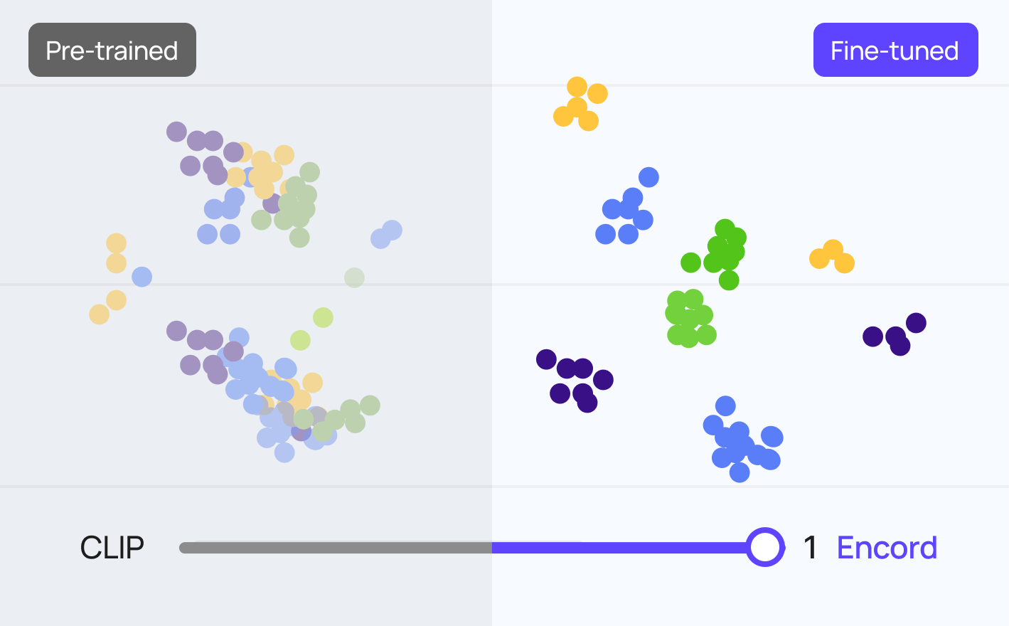
As the world generates an ever-expanding volume of visual content, the need for efficient data curation becomes increasingly important. Whether it’s satellite imagery, aerial photographs, or remote sensing data, organizing and annotating these visuals is essential for scientific research, urban planning, disaster response, and more. In this blog post, we explore how fine-tuning the Contrastive Language-Image Pre-Training or CLIP model with the RSICD dataset—a collection of remote sensing images and captions—revolutionizes how we curate geospatial data. Unlike traditional image processing methods, CLIP offers advanced capabilities like semantic search and multilingual annotations, improving the processing and analysis of geospatial information. Fine-Tuning Vision-Language Models (VLMs) Fine-tuning Vision-Language Models (VLM) to enhance embeddings is a cutting-edge approach to data curation. VLMs are advanced models that combine visual and textual understanding, making them incredibly powerful tools for processing and analyzing multimedia data. By fine-tuning these models specifically for geospatial tasks, we aim to improve the accuracy and efficiency of location-based data processing and analysis. Geo-spatial Embeddings Geo-spatial embeddings refer to representations of geographical locations in a continuous vector space, where each location is encoded as a vector with semantic meaning. These embeddings are crucial for various applications such as geographical information systems (GIS), location-based recommendation systems, urban planning, environmental monitoring, and disaster response, among others. However, generating accurate geospatial embeddings from heterogeneous data sources poses significant challenges due to the complexity and diversity of spatial information. At Encord, we address these challenges by fine-tuning VLMs like CLIP to produce more accurate and semantically rich geospatial embeddings. This can help streamline your data curation process with new possibilities in how you use geospatial data. Importance of Fine-Tuning VLM in Data Curation The importance of fine-tuning VLMs in data curation can be understood through several key aspects: Semantic Understanding VLMs are capable of understanding and interpreting both visual and textual information simultaneously. By fine-tuning these models on specific datasets relevant to a particular domain, such as medical imaging or satellite imagery, they can learn to associate visual features with corresponding textual descriptions. This semantic understanding greatly enriches the curated data by providing context and meaning to the information being processed. So the annotators can quickly identify and tag images based on textual descriptions, improving dataset organization and curation. Adaptability to Domain-Specific Requirements Different domains have unique data characteristics and requirements. Fine-tuning VLMs allows for customization and adaptation to these domain-specific needs. For example, here we are fine-tuning the VLM model to improve geospatial embeddings. Improved Data Accuracy Fine-tuning VLMs enables them to better capture the complexities of the data being curated. This results in improved relevance and accuracy of the curated datasets as the models learn to extract and highlight the most relevant features and information. Consequently, curated datasets become more valuable for downstream tasks such as machine learning, analytics, and decision-making processes. Fine-Tuning CLIP with RSICD CLIP Contrastive Language-Image Pre-training or CLIP, developed by OpenAI, is a powerful multimodal model that bridges the gap between natural language and visual content. It learns to associate images and their corresponding captions in a self-supervised manner, enabling it to perform tasks like image search, zero-shot classification, and more. RSICD Dataset The Remote Sensing Image Caption Dataset or RSICD serves as our training ground. Comprising approximately 10,000 satellite images, this dataset features both image labels and descriptive captions. These captions provide valuable context, making RSICD an ideal candidate for fine-tuning CLIP. Why Fine-Tune CLIP with RSICD? Geo-Spatial Specificity Satellite images differ significantly from everyday photos. Captured by orbiting satellites, differ from normal ground-level images in scale, perspective, and resolution. By fine-tuning CLIP with RSICD, we tailor the model to understand the complexities of geospatial data. This specificity enhances its ability to handle satellite imagery effectively. Strengthen Search Ability By incorporating captions during fine-tuning, we ensure that the model embeds both image and text information cohesively. Consequently, CLIP becomes adept at natural language search and image retrieval. Embedding Space Before Fine-Tuning. The scattered arrangement of clusters represents data points in the initial embedding space. Embedding Space After Fine-Tuning. A more refined and cohesive grouping of data points indicates an improved embedding space post-fine-tuning. Zero-Shot Performance Evaluation We evaluate the model’s zero-shot performance using ground truth labels. This involves assessing whether the textual embeddings align with the image embeddings. Such alignment validates the consistency of CLIP’s image-text capabilities. Significance of Fine-Tuning CLIP with RSICD Geo-Spatial Annotation Precision Contextual Understanding: RSICD provides satellite images alongside descriptive captions. By fine-tuning CLIP, we enhance its ability to understand the nuances of geospatial features—mountains, rivers, forests, urban areas, and more. Accurate Labeling: Curators can annotate images with greater precision. Whether identifying specific land cover types or pinpointing landmarks, CLIP ensures context-aware annotations. Efficient Data Exploration Semantic Search: Curators and researchers can query the dataset using natural language. CLIP retrieves relevant images based on textual descriptions. For instance, searching for “coastal erosion” yields coastal satellite imagery. Time Savings: Manual exploration of thousands of images becomes streamlined. CLIP acts as a smart filter, presenting relevant visuals promptly. Consistent Labeling and Quality Control Alignment of Embeddings: During fine-tuning, CLIP learns to align image embeddings with textual embeddings. Curators can cross-check whether the textual descriptions match the visual content. Uniform Annotations: Consistent labeling improves model training and downstream tasks. Whether detecting deforestation or urban sprawl, CLIP ensures uniformity. In summary, fine-tuning CLIP with RSICD empowers data curators by providing efficient search, consistent labeling, multilingual support, and domain-specific expertise. As we embrace this powerful tool, we pave the way for smarter, more accessible datasets.
April 4
5 min

What is YOLO Object Detection? YOLO (You Only Look Once) models are real-time object detection systems that identify and classify objects in a single pass of the image. What is Object Detection? Object detection is a critical capability of computer vision that identifies and locates objects within an image or video. Unlike image classification, object detection not only classifies the objects in an image, but also identifies their location within the image by drawing a bounding box around each object. Object detection models, such as R-CNN, Fast R-CNN, Faster R-CNN, and YOLO, use convolutional neural networks (CNNs) to classify the objects and regressor networks to accurately predict the bounding box coordinates for each detected object. Image Classification Image classification is a fundamental task in computer vision. Given an input image, the goal of an image classification model is to assign it to one of a pre-defined set of classes. Most image classification models use CNNs, which are specifically designed to process pixel data and can capture spatial features. Image classification models are trained on large datasets (like ImageNet) and can classify images into 1000 object categories, such as keyboard, mouse, pencil, and many animals. Object Localization Object localization is another important task in computer vision that identifies the location of an object in the image. It extends the image classification model by adding a regression head to predict the bounding box coordinates of the object. The bounding box is typically represented by four coordinates that define its position and size. Object localization is a key step in object detection, where the goal is not just to classify the primary object of interest in the image, but also to identify its location. Classification of Object Detection Algorithms Object detection algorithms can be broadly classified into two categories: single-shot detectors and two-shot(or multi-shot) detectors. These two types of algorithms have different approaches to the task of object detection. Single-Shot Object Detection Single-shot detectors (SSDs) are a type of object detection algorithm that predict the bounding box and the class of the object in one single shot. This means that in a single forward pass of the network, the presence of an object and the bounding box are predicted simultaneously. This makes SSDs very fast and efficient, suitable for tasks that require real-time detection. Structure of SSD Examples of single-shot object detection algorithms include YOLO (You Only Look Once) and SSD (Single Shot MultiBox Detector). YOLO divides the input image into a grid and for each grid cell, predicts a certain number of bounding boxes and class probabilities. SSD, on the other hand, predicts bounding boxes and class probabilities at multiple scales in different feature maps. Two-Shot Object Detection Two-shot or multi-shot object detection algorithms, on the other hand, use a two-step process for detecting objects. The first step involves proposing a series of bounding boxes that could potentially contain an object. This is often done using a method called region proposal. The second step involves running these proposed regions through a convolutional neural network to classify the object classes within the box. Examples of two-shot object detection algorithms include R-CNN (Regions with CNN features), Fast R-CNN, and Faster R-CNN. These algorithms use region proposal networks (RPNs) to propose potential bounding boxes and then use CNNs to classify the proposed regions. Both single-shot and two-shot detectors have their strengths and weaknesses. Single-shot detectors are generally faster and more efficient, making them suitable for real-time object detection tasks. Two-shot detectors, while slower and more computationally intensive, tend to be more accurate, as they can afford to spend more computational resources on each potential object. Object Detection Methods Object Detection: Non-Neural Methods Viola-Jones object detection method based on Haar features The Viola-Jones method, introduced by Paul Viola and Michael Jones, is a machine learning model for object detection. It uses a cascade of classifiers, selecting features from Haar-like feature sets. The algorithm has four stages: Haar Feature Selection Creating an Integral Image Adaboost Training Cascading Classifiers Despite its simplicity and speed, it can achieve high detection rates. Scale-Invariant Feature Transform (SIFT) SIFT is a method for extracting distinctive invariant features from images. These features are invariant to image scale and rotation, and are robust to changes in viewpoint, noise, and illumination. SIFT features are used to match different views of an object or scene. Histogram of Oriented Gradients (HOG) HOG is a feature descriptor used for object detection in computer vision. It involves counting the occurrences of gradient orientation in localized portions of an image. This method is similar to edge orientation histograms, scale-invariant feature transform descriptors, and shape contexts, but differs in that it is computed on a dense grid of uniformly spaced cells. Object Detection: Neural Methods Region-Based Convolutional Neural Networks (R-CNN) Region-Based CNN uses convolutional neural networks to classify image regions in order to detect objects. It involves training a CNN on a large labeled dataset and then using the trained network to detect objects in new images. Region-Based CNN and its successors, Fast R-CNN and Faster R-CNN, are known for their accuracy but can be computationally intensive. Faster R-CNN Faster R-CNN is an advanced version of R-CNN that introduces a Region Proposal Network (RPN) for generating region proposals. The RPN shares full-image convolutional features with the detection network, thus enabling nearly cost-free region proposals. The RPN is a fully convolutional network that simultaneously predicts object bounds and objectness scores at each position. Faster R-CNN is faster than the original R-CNN and Fast R-CNN because it doesn’t need to run a separate region proposal method on the image, which can be slow. Mask R-CNN Mask R-CNN extends Faster R-CNN by adding a branch for predicting an object mask in parallel with the existing branch for bounding box recognition. This allows Mask R-CNN to generate precise segmentation masks for each detected object, in addition to the class label and bounding box. The mask branch is a small fully convolutional network applied to each RoI, predicting a binary mask for each RoI. Mask R-CNN is simple to train and adds only a small computational overhead, enabling a fast system and rapid experimentation. Single Shot Detector (SSD) SSD is a method for object detection that eliminates the need for multiple network passes for multiple scales. It discretizes the output space of bounding boxes into a set of default boxes over different aspect ratios and scales per feature map location. SSD is faster than methods like R-CNN because it eliminates bounding box proposals and pooling layers. RetinaNet RetinaNet uses a feature pyramid network on top of a backbone to detect objects at different scales and aspect ratios. It introduces a new loss, the Focal Loss, to deal with the foreground-background class imbalance problem. RetinaNet is designed to handle dense and small objects. EfficientDet EfficientDet is a method that scales all dimensions of the network width, depth, and resolution with a compound scaling method to achieve better performance. It introduces a new architecture, called BiFPN, which allows easy and efficient multi-scale feature fusion, and a new scaling method that uniformly scales the resolution, depth, and width for all backbone, feature network, and box/class prediction networks at the same time. EfficientDet achieves state-of-the-art accuracy with fewer parameters and less computation compared to previous detectors. You Only Look Once (YOLO) YOLO, developed by Joseph Redmon et al., frames object detection as a regression problem to spatially separated bounding boxes and associated class probabilities. It looks at the whole image at test time so its predictions are informed by global context in the image. YOLO is known for its speed, making it suitable for real-time applications. You Only Look Once: Unified, Real-Time Object Detection Object Detection: Performance Evaluation Metrics Intersection over Union (IoU) IoU (Intersection over Union) Calculation Intersection over Union (IoU) is a common metric used to evaluate the performance of an object detection algorithm. It measures the overlap between the predicted bounding box (P) and the ground truth bounding box (G). The IoU is calculated as the area of intersection divided by the area of union of P and G. The IoU score ranges from 0 to 1, where 0 indicates no overlap and 1 indicates a perfect match. A higher IoU score indicates a more accurate object detection. Average Precision (AP) Average Precision (AP) is another important metric used in object detection. It summarizes the precision-recall curve that is created by varying the detection threshold. Precision is the proportion of true positive detections among all positive detections, while recall is the proportion of true positive detections among all actual positives in the image. The AP computes the average precision values for recall levels over 0 to 1. The AP score ranges from 0 to 1, where a higher value indicates better performance. The mean Average Precision (mAP) is often used in practice, which calculates the AP for each class and then takes the average. By understanding these metrics, we can better interpret the performance of models like YOLO and make informed decisions about their application in real-world scenarios. After exploring various object detection methods and performance evaluation methods, let’s delve into the workings of a particularly powerful and popular algorithm known as ‘You Only Look Once’, or YOLO. This algorithm has revolutionized the field of object detection with its unique approach and impressive speed. Unlike traditional methods that involve separate steps for identifying objects and classifying them, YOLO accomplishes both tasks in a single pass, hence the name ‘You Only Look Once’. YOLO Object Detection Algorithm: How Does it Work? YOLO Architecture The YOLO algorithm employs a single Convolutional Neural Network (CNN) that divides the image into a grid. Each cell in the grid predicts a certain number of bounding boxes. Along with each bounding box, the cell also predicts a class probability, which indicates the likelihood of a specific object being present in the box. Convolution Layers Bounding Box Recognition Process The bounding box recognition process in YOLO involves the following steps: Grid Creation: The image is divided into an SxS grid. Each grid cell is responsible for predicting an object if the object’s center falls within it. Bounding Box Prediction: Each grid cell predicts B bounding boxes and confidence scores for those boxes. The confidence score reflects how certain the model is that a box contains an object and how accurate it thinks the box is. Class Probability Prediction: Each grid cell also predicts C conditional class probabilities (one per class for the potential objects). These probabilities are conditioned on there being an object in the box. YOLO Structure Non-Max Suppression (NMS) After the bounding boxes and class probabilities are predicted, post-processing steps are applied. One such step is Non-Max Suppression (NMS). NMS helps in reducing the number of overlapping bounding boxes. It works by eliminating bounding boxes that have a high overlap with the box that has the highest confidence score. Vector Generalization Vector generalization is a technique used in the YOLO algorithm to handle the high dimensionality of the output. The output of the YOLO algorithm is a tensor that contains the bounding box coordinates, objectness score, and class probabilities. This high-dimensional tensor is flattened into a vector to make it easier to process. The vector is then passed through a softmax function to convert the class scores into probabilities. The final output is a vector that contains the bounding box coordinates, objectness score, and class probabilities for each grid cell. Evolution of YOLO: YOLOv1, YOLOv2, YOLOv3, YOLOv4, YOLOR, YOLOX, YOLOv5, YOLOv6, YOLOv7, YOLOv8, YOLOv9 If you are not interested in a quick recap of the timeline of YOLO models and the updates in the network architecture, skip this section! YOLOv1: First Real-time Object Detection Algorithm The original YOLO model treated object detection as a regression problem, which was a significant shift from the traditional classification approach. It used a single convolutional neural network (CNN) to detect objects in images by dividing the image into a grid, making multiple predictions per grid cell, filtering out low-confidence predictions, and then removing overlapping boxes to produce the final output. YOLOv2 [YOLO9000]: Multi-Scale Training| Anchor Boxes| Darknet-19 Backbone YOLOv2 introduced several improvements over the original YOLO. It used batch normalization in all its convolutional layers, which reduced overfitting and improved model stability and performance. It could handle higher-resolution images, making it better at spotting smaller objects. YOLOv2 also used anchor boxes (borrowed from Faster R-CNN), which helped the algorithm predict the shape and size of objects more accurately. YOLOv3: Three YOLO Layers| Logistic Classifiers| Upsampling |Darknet-53 Backbone Upsampling YOLOv3 introduced a new backbone network, Darknet-53, which utilized residual connections. It also made several design changes to improve accuracy while maintaining speed. At 320x320 resolution, YOLOv3 ran in 22 ms at 28.2 mAP, as accurate as SSD but three times faster. It achieved 57.9 mAP@50 in 51 ms on a Titan X, compared to 57.5 mAP@50 in 198 ms by RetinaNet, with similar performance but 3.8x faster. YOLOv4: CSPDarknet53 | Detection Across Scales | CIOU Loss Speed Comparison: YOLOv4 Vs. YOLOv3 YOLOv4 introduced several new techniques to improve both accuracy and speed. It used a CSPDarknet backbone and introduced new techniques such as spatial attention, Mish activation function, and GIoU loss to improve accuracy3. The improved YOLOv4 algorithm showed a 0.5% increase in average precision (AP) compared to the original algorithm while reducing the model’s weight file size by 45.3 M. YOLOR: Unified Network Architecture | Mosaic | Mixup | SimOTA UNA (Unified Network Architecture) Unlike previous YOLO versions, YOLOR’s architecture and model infrastructure differ significantly. The name “YOLOR” emphasizes its unique approach: it combines explicit and implicit knowledge to create a unified network capable of handling multiple tasks with a single input. By learning just one representation, YOLOR achieves impressive performance in object detection. YOLOX YOLOX is an anchor-free object detection model that builds upon the foundation of YOLOv3 SPP with a Darknet53 backbone. It aims to surpass the performance of previous YOLO versions. The key innovation lies in its decoupled head and SimOTA approach. By eliminating anchor boxes, YOLOX simplifies the design while achieving better accuracy. It bridges the gap between research and industry, offering a powerful solution for real-time object detection. YOLOX comes in various sizes, from the lightweight YOLOX-Nano to the robust YOLOX-x, each tailored for different use cases. YOLOv5: PANet| CSPDarknet53| SAM Block YOLOv5 brought about further enhancements to increase both precision and efficiency. It adopted a Scaled-YOLOv4 backbone and incorporated new strategies such as CIOU loss and CSPDarknet53-PANet-SPP to boost precision. Structure of YOLOv5 The refined YOLOv5 algorithm demonstrated a 0.7% rise in mean average precision (mAP) compared to the YOLOv4, while decreasing the model’s weight file size by 53.7 M. These improvements made YOLOv5 a more effective and efficient tool for real-time object detection. YOLOv6: EfficientNet-Lite | CSPDarknet-X backbone | Swish Activation Function | DIoU Loss YOLOv6 utilized a CSPDarknet-X backbone and introduced new methods such as panoptic segmentation, Swish activation function, and DIoU loss to boost accuracy. Framework of YOLOv6 The enhanced YOLOv6 algorithm exhibited a 0.8% increase in average precision (AP) compared to the YOLOv5, while shrinking the model’s weight file size by 60.2 M. These advancements made YOLOv6 an even more powerful tool for real-time object detection. YOLOv7: Leaky ReLU Activation Function| TIoU Loss| CSPDarknet-Z Backbone YOLOv7 employed a CSPDarknet-Z backbone in the yolov7 architecture. YOLOv7 object detection algorithm was enhanced by the introduction of innovative techniques such as object-centric segmentation, Leaky ReLU activation function, and TIoU loss to enhance accuracy. The advanced YOLOv7 algorithm demonstrated a 1.0% increase in average precision (AP) compared to the YOLOv6, while reducing the model’s weight file size by 70.5 M. These improvements made YOLOv7 object detection algorithm, an even more robust tool for real-time object detection. YOLOv8: Multi-Scale Object Detection| CSPDarknet-AA| ELU Activation Function| GIoU Loss YOLOv8 introduced a new backbone architecture, the CSPDarknet-AA, which is an advanced version of the CSPDarknet series, known for its efficiency and performance in object detection tasks. One key technique introduced in YOLOv8 is multi-scale object detection. This technique allows the model to detect objects of various sizes in an image. Another significant enhancement in YOLOv8 is the use of the ELU activation function. ELU, or Exponential Linear Unit, helps to speed up learning in deep neural networks by mitigating the vanishing gradient problem, leading to faster convergence. YOLOv8 adopted the GIoU loss. GIoU, or Generalized Intersection over Union, is a more advanced version of the IoU (Intersection over Union) metric that takes into account the shape and size of the bounding boxes, improving the precision of object localization. The YOLOv8 algorithm shows a 1.2% increase in average precision (AP) compared to the YOLOv7, which is a significant improvement. It has achieved this while reducing the model’s weight file size by 80.6 M, making the model more efficient and easier to deploy in resource-constrained environments. YOLOv8 Comparison with Latest YOLO models YOLOv9: GELAN Architecture| Programmable Gradient Information (PGI) YOLOv9 which was recently released overcame information loss challenges inherent in deep neural networks. By integrating PGI and the versatile GELAN architecture, YOLOv9 not only enhances the model’s learning capacity but also ensures the retention of crucial information throughout the detection process, thereby achieving exceptional accuracy and performance. Key Highlights of YOLOv9 Information Bottleneck Principle: This principle reveals a fundamental challenge in deep learning: as data passes through successive layers of a network, the potential for information loss increases. YOLOv9 counters this challenge by implementing Programmable Gradient Information (PGI), which aids in preserving essential data across the network’s depth, ensuring more reliable gradient generation and, consequently, better model convergence and performance. Reversible Functions: A function is deemed reversible if it can be inverted without any loss of information. YOLOv9 incorporates reversible functions within its architecture to mitigate the risk of information degradation, especially in deeper layers, ensuring the preservation of critical data for object detection tasks. For more information, read the blog YOLOv9: SOTA Object Detection Model Explained. YOLO Object Detection with Pre-Trained YOLOv9 on COCO Dataset Like all YOLO models, the pre-trained models of YOLOv9 is open-source and is available in GitHub. We are going to run our experiment on Google Colab. So if you are doing it on your local system, please bear in mind that the instructions and the code was made to run on Colab Notebook. Make sure you have access to GPU. You can either run the command below or navigate to Edit → Notebook settings → Hardware accelerator, set it to GPU, and the click Save. !nvidia-smi To make it easier to manage datasets, images, and models we create a HOME constant. import os HOME = os.getcwd() print(HOME) Clone and Install !git clone https://github.com/SkalskiP/yolov9.git %cd yolov9 !pip install -r requirements.txt -q Download Model Weights !wget -P {HOME}/weights -q https://github.com/WongKinYiu/yolov9/releases/download/v0.1/yolov9-c.pt !wget -P {HOME}/weights -q https://github.com/WongKinYiu/yolov9/releases/download/v0.1/yolov9-e.pt !wget -P {HOME}/weights -q https://github.com/WongKinYiu/yolov9/releases/download/v0.1/gelan-c.pt !wget -P {HOME}/weights -q https://github.com/WongKinYiu/yolov9/releases/download/v0.1/gelan-e.pt Test Data Upload test image to the Colab notebook. !wget -P {HOME}/data -q –-add image path Detection with Pre-trained COCO Model on gelan-c !python detect.py --weights {HOME}/weights/gelan-c.pt --conf 0.1 --source image path --device 0 Evaluation of the Pre-trained COCO Model on gelan-c !python val.py --data data/coco.yaml --img 640 --batch 32 --conf 0.001 --iou 0.7 --device 0 --weights './gelan-c.pt' --save-json --name gelan_c_640_val Performance of YOLOv9 on MS COCO Dataset Yolov9: Learning What You Want to Learn Using Programmable Gradient Information The performance of YOLOv9 on the MS COCO dataset exemplifies its significant advancements in real-time object detection, setting new benchmarks across various model sizes. The smallest of the models, v9-S, achieved 46.8% AP on the validation set of the MS COCO dataset, while the largest model, v9-E, achieved 55.6% AP. This sets a new state-of-the-art for object detection performance. These results demonstrate the effectiveness of YOLOv9’s techniques, such as Programmable Gradient Information (PGI) and the Generalized Efficient Layer Aggregation Network (GELAN), in enhancing the model’s learning capacity and ensuring the retention of crucial information throughout the detection process. For more information, read the paper of Arxiv: Yolov9: Learning What You Want to Learn Using Programmable Gradient Information. Training YOLOv9 on Custom Dataset Here for training data, we will be curating a custom dataset on Encord platform. With Encord you can either curate and create your custom dataset or use the sandbox datasets already created on Encord Active platform. Select New Dataset to Upload Data You can name the dataset and add a description to provide information about the dataset. Annotate Custom Dataset Create an annotation project and attach the dataset and the ontology to the project to start annotation with a workflow. You can choose manual annotation if the dataset is simple, small, and doesn’t require a review process. Automated annotation is also available and is very helpful in speeding up the annotation process. For more information on automated annotation, read the blog The Full Guide to Automated Data Annotation. Start Labeling The summary page shows the progress of the annotation project. The information regarding the annotators and the performance of the annotators can be found under the tabs labels and performance. Export the Annotation Once the annotation has been reviewed, export the annotation in the required format. For more information on exploring the quality of your custom dataset, read the blog Exploring the Quality of Hugging Face Image Datasets with Encord Active. You can use the custom dataset curated using Encord Annotate for training an object detection model. For testing YOLOv9, we are going to use an image from one of the sandbox projects on Encord Active. Copy and run the code below to run YOLOv9 for object detection. The code for using YOLOv9 for panoptic segmentation has also been made available now on the original GitHub repository. Installing YOLOv9 !git clone https://github.com/SkalskiP/yolov9.git %cd yolov9 !pip install -r requirements.txt -q !pip install -q roboflow encord av # This is a convenience class that holds the info about Encord projects and makes everything easier. # The class supports bounding boxes and polygons across both images, image groups, and videos. !wget 'https://gist.githubusercontent.com/frederik-encord/e3e469d4062a24589fcab4b816b0d6ec/raw/fa0bfb0f1c47db3497d281bd90dd2b8b471230d9/encord_to_roboflow_v1.py' -O encord_to_roboflow_v1.py Imports from typing import Literal from pathlib import Path from IPython.display import Image import roboflow from encord import EncordUserClient from encord_to_roboflow_v1 import ProjectConverter Download YOLOv9 Model Weights The YOLOv9 is available as 4 models which are ordered by parameter count: YOLOv9-S YOLOv9-M YOLOv9-C YOLOv9-E Here we will be using gelan-c. But the same process follows for other models. !mkdir -p {HOME}/weights !wget -q https://github.com/WongKinYiu/yolov9/releases/download/v0.1/yolov9-e-converted.pt -O {HOME}/weights/yolov9-e.pt !wget -P {HOME}/weights -q https://github.com/WongKinYiu/yolov9/releases/download/v0.1/gelan-c.pt Train Custom YOLOv9 Model for Object Detection !python train.py \ --batch 8 --epochs 20 --img 640 --device 0 --min-items 0 --close-mosaic 15 \ --data $dataset_yaml_file \ --weights {HOME}/weights/gelan-c.pt \ --cfg models/detect/gelan-c.yaml \ --hyp hyp.scratch-high.yaml For more information on end-to-end training YOLOv9 with custom dataset, check out the blog Comparative Analysis of YOLOv9 and YOLOv8 Using Custom Dataset on Encord Active. YOLO Object Detection using YOLOv9 on Custom Dataset In order to perform object detection, you have to run prediction of the trained YOLOv9 on custom dataset. Run Prediction import torch augment = False visualize = False conf_threshold = 0.25 nms_iou_thres = 0.45 max_det = 1000 seen, windows, dt = 0, [], (Profile(), Profile(), Profile()) for path, im, im0s, vid_cap, s in dataset: with dt[0]: im = torch.from_numpy(im).to(model.device).float() im /= 255 # 0 - 255 to 0.0 - 1.0 if len(im.shape) == 3: im = im[None] # expand for batch dim # Inference with dt[1]: pred = model(im, augment=augment, visualize=visualize)[0] # NMS with dt[2]: filtered_pred = non_max_suppression(pred, conf_threshold, nms_iou_thres, None, False, max_det=max_det) print(pred, filtered_pred) break Generate YOLOv9 Prediction on Custom Data import matplotlib.pyplot as plt from matplotlib.patches import Rectangle from PIL import Image img = Image.open(Image path) fig, ax = plt.subplots() ax.imshow(img) ax.axis("off") for p, c in zip(filtered_pred[0], ["r", "b", "g", "cyan"]): x, y, w, h, score, cls = p.detach().cpu().numpy().tolist() ax.add_patch(Rectangle((x, y), w, h, color="r", alpha=0.2)) ax.text(x+w/2, y+h/2, model.names[int(cls)], ha="center", va="center", color=c) fig.savefig("/content/predictions.jpg") YOLOv9 Vs YOLOv8: Comparative Analysis Using Encord You can convert the model predictions and upload them to Encord. Here for example, the YOLOv9 and YOLOv8 have been trained and compared on the Encord platform using the xView3 dataset, which contains aerial imagery with annotations for maritime object detection. The comparative analysis between YOLOv9 and YOLOv8 on the Encord platform focuses on precision, recall, and metric analysis. These metrics are crucial for evaluating the performance of object detection models. Precision: Precision measures the proportion of true positives (i.e., correct detections) among all detections. A higher precision indicates fewer false positives. Recall: Recall measures the proportion of actual positives that are correctly identified. A higher recall indicates fewer false negatives. Metric Analysis: This involves analyzing various metrics like Average Precision (AP), Mean Average Precision (mAP), etc., which provide a comprehensive view of the model’s performance. For example, in the precision-recall curve, it seems that YOLOv8 surpasses YOLOv9 in terms of the Area Under the Curve (AUC-PR) value. This suggests that, across various threshold values, YOLOv8 typically outperforms YOLOv9 in both precision and recall. It implies that YOLOv8 is more effective at correctly identifying true positives and reducing false positives compared to YOLOv9. But it is important to keep in mind that these two models which are being evaluated were trained for 20 epochs and are used as an example to show how to perform evaluation of trained models on custom datasets. For detailed information on performing a comparative analysis of trained models, read the blog Comparative Analysis of YOLOv9 and YOLOv8 Using Custom Dataset on Encord Active. YOLO Real-Time Implementation YOLO (You Only Look Once) models are widely used in real-time object detection tasks due to their speed and accuracy. Here are some real-world applications of YOLO models: Healthcare: YOLO models can be used in healthcare for tasks such as identifying diseases or abnormalities in medical images. Agriculture: YOLO models have been used to detect and classify crops, pests, and diseases, assisting in precision agriculture techniques and automating farming processes. Security Surveillance: YOLO models are used in security surveillance systems for real-time object detection, tracking, and classification. Self-Driving Cars: In autonomous vehicles, YOLO models are used for detecting objects such as other vehicles, pedestrians, traffic signs, and signals in real-time. Face Detection: They have also been adapted for face detection tasks in biometrics, security, and facial recognition systems YOLO Object Detection: Key Takeaways In this article, we provided an overview of the evolution of YOLO, from YOLOv1 to YOLOv8, and discussed its network architecture, new features, and applications. Additionally, we provided a step-by-step guide on how to use YOLOv8 for object detection and how to create model-assisted annotations with Encord Annotate. At Encord, we help computer vision companies build better models and training datasets. We have built an end-to-end Active Learning Platform for AI-assisted annotation workflows evaluating and evaluating your training data Orchestrating active learning pipelines Fixing data and label errors Diagnosing model errors & biases. Encord integrates the new YOLOv8 state-of-the-art model and allows you to train Micro-models on a backbone of YOLOv8 models to support your AI-assisted annotation work.
April 4
7 min
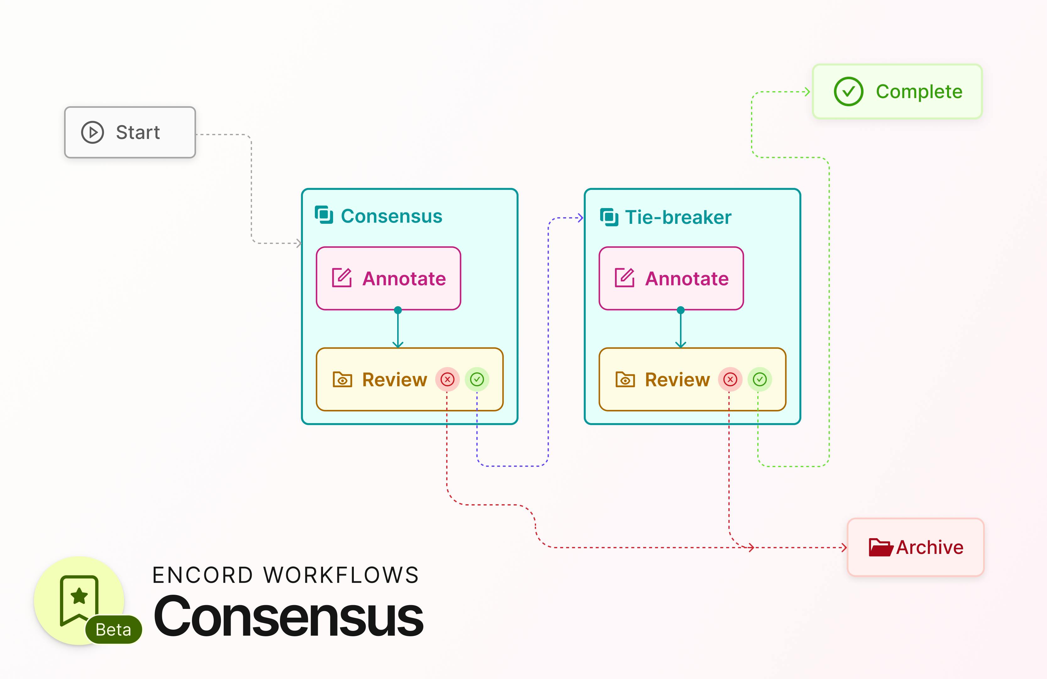
At Encord, we continually obsess over how to support ML teams managing their labeling workflows and make it as easy as possible for teams to improve model performance. Today, we’re announcing the launch of Consensus workflows within Encord. What is Consensus? Consensus allows multiple annotators to conduct a labeling task of the same file in a mutually blind fashion — that is, each annotator is unaware that other annotators are working on the task. All submissions are aggregated into the following evaluation substage where designated Consensus reviewers can evaluate the agreement between labels and select a representative set. Integrating Consensus into your labeling workflows allows you to create higher-quality annotations by assessing the submissions of multiple annotators and simplifying compliance with domain-specific regulatory requirements. Support within Encord Support will begin with image and video modalities, with full modality support progressively released soon after. You can read more in our documentation for more information on activating this feature and building consensus workflows.
April 2
2 min
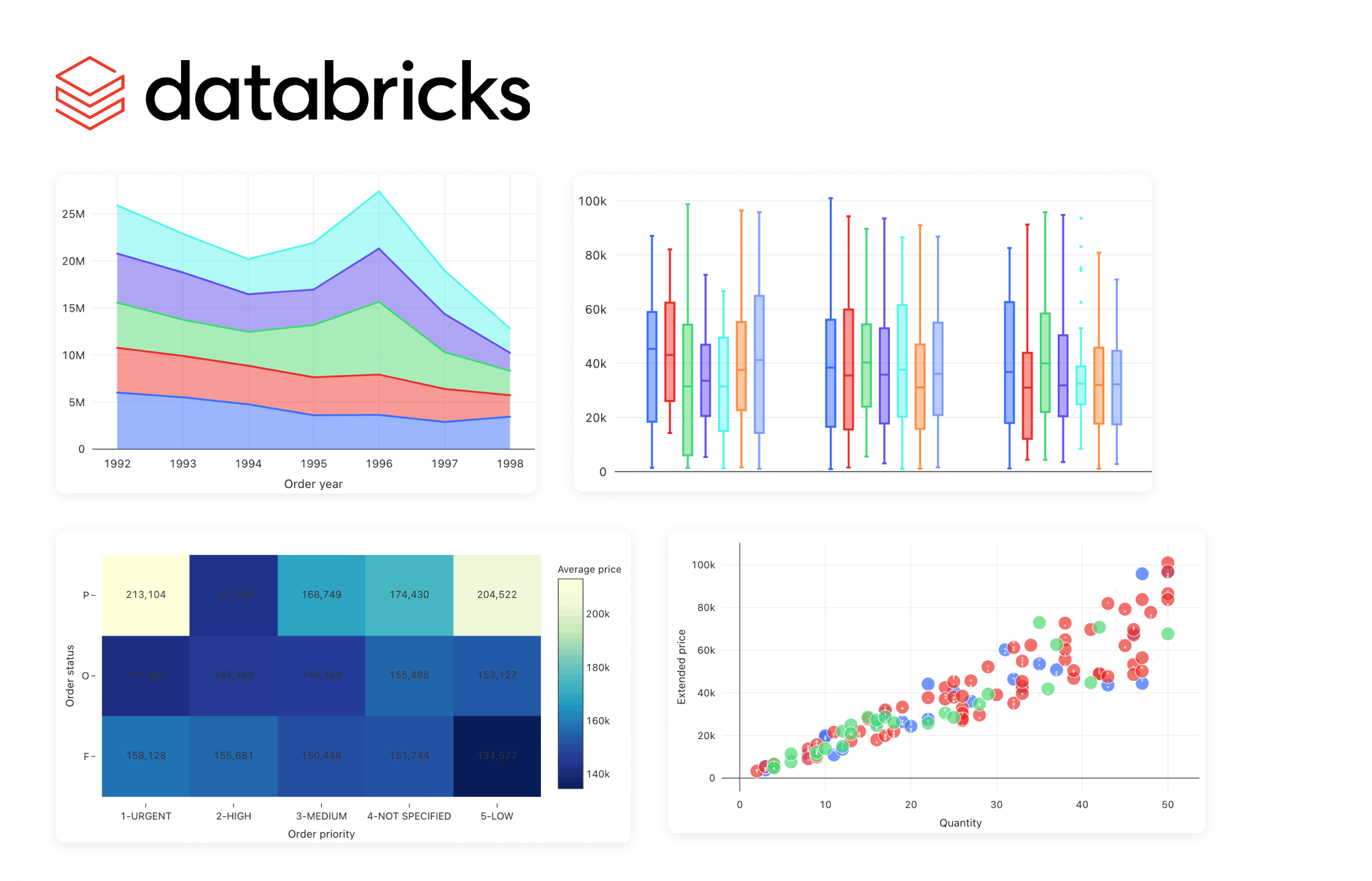
With data becoming a pillar stone of a company’s growth strategy, the market for visualization tools is growing rapidly, with a projected compound annual growth rate (CAGR) of 10.07% between 2023 and 2028. The primary driver of these trends is the need for data-driven decision-making, which involves understanding complex data patterns and extracting actionable insights to improve operational efficiency. PowerBI and Tableau are traditional tools with interactive workspaces for creating intuitive dashboards and exploring large datasets. However, other platforms are emerging to address the ever-changing nature of the modern data ecosystem. In this article, we will discuss the visualizations offered by Databricks - a modern enterprise-scale platform for building data, analytics, and artificial intelligence (AI) solutions. Databricks Databricks is an end-to-end data management and model development solution built on Apache Spark. It lets you create and deploy the latest generative AI (Gen AI) and large language models (LLMs). The platform uses a proprietary Mosaic AI framework to streamline the model development process. It provides tools to fine-tune LLMs seamlessly through enterprise data and offers a unified service for experimentation through foundation models. In addition, it features Databricks SQL, a state-of-the-art lakehouse for cost-effective data storage and retrieval. It lets you centrally store all your data assets in an open format, Delta Lake, for effective governance and discoverability. Further, Databricks SQL has built-in support for data visualization, which lets you extract insights from datasets directly from query results in the SQL editor. Users also benefit from the visualization tools featured in Databricks Notebooks, which help you build interactive charts by using the Plotly library in Python. Through these visualizations, Databricks offers robust data analysis for monitoring data assets critical to your AI models. So, let’s discuss in more detail the types of chart visualizations, graphs, diagrams, and maps available on Databricks to help you choose the most suitable visualization type for your use case. Effective visualization can help with effortless data curation. Learn more about how you can use data curation for computer vision Visualizations in Databricks As mentioned earlier, Databricks provides visualizations through Databricks SQL and Databricks Notebooks. The platform lets you run multiple SQL queries to perform relevant aggregations and apply filters to visualize datasets according to your needs. Databricks also allows you to configure settings related to the X and Y axes, legends, missing values, colors, and labels. Users can also download visualizations in PNG format for documentation purposes. The following sections provide an overview of the various visualization types available in these two frameworks, helping you select the most suitable option for your project. Bar Chart Bar charts are helpful when you want to compare the frequency of occurrence of different categories in your dataset. For instance, you can draw a bar chart to compare the frequency of various age groups, genders, ethnicities, etc. Additionally, bar charts can be used to view the sum of the prices of all orders placed in a particular month and group them by priority. Bar chart The result will show the months on the X-axis and the sum of all the orders categorized by priority on the Y-axis. Line Line charts connect different data points through straight lines. They are helpful when users want to analyze trends over some time. The charts usually show time on the X-axis and some metrics whose trajectory you want to explore on the Y-axis. Line chart For instance, you can view changes in the average price of orders over the years grouped by priority. The trends can help you predict the most likely future values, which can help you with financial projections and budget planning. Pie Chart Pie charts display the proportion of different categories in a dataset. They divide a circle into multiple segments, each showing the proportion of a particular category, with the segment size proportional to the category’s percentage of the total. Pie chart For instance, you can visualize the proportion of orders for each priority. The visualization is helpful when you want a quick overview of data distribution across different segments. It can help you analyze demographic patterns, market share of other products, budget allocation, etc. Scatter Plot A scatter plot displays each data point as a dot representing a relationship between two variables. Users can also control the color of each dot to reflect the relationship across different groups. Scatter Plot For instance, you can plot the relationship between quantity and price for different color-coded item categories. The visualization helps in understanding the correlation between two variables. However, users must interpret the relationship cautiously, as correlation does not always imply causation. Deeper statistical analysis is necessary to uncover causal factors. Area Charts Area charts combine line and bar charts by displaying lines and filling the area underneath with colors representing particular categories. They show how the contribution of a specific category changes relative to others over time. Area Charts For instance, you can visualize which type of order priority contributed the most to revenue by plotting the total price of different order priorities across time. The visualization helps you analyze the composition of a specific metric and how that composition varies over time. It is particularly beneficial in analyzing sales growth patterns for different products, as you can see which product contributed the most to growth across time. Box Chart Box charts concisely represent data distributions of numerical values for different categories. They show the distribution’s median, skewness, interquartile, and value ranges. Box Chart For instance, the box can display the median price value through a line inside the box and the interquartile range through the top and bottom box enclosures. The extended lines represent minimum and maximum price values to compute the price range. The chart helps determine the differences in distribution across multiple categories and lets you detect outliers. You can also see the variability in values across different categories and examine which category was the most stable. Bubble Chart Bubble charts enhance scatter plots by allowing you to visualize the relationship of three variables in a two-dimensional grid. The bubble position represents how the variable on the X-axis relates to the variable on the Y-axis. The bubble size represents the magnitude of a third variable, showing how it changes as the values of the first two variables change. Bubble chart The visualization is helpful for multi-dimensional datasets and provides greater insight when analyzing demographic data. However, like scatter plots, users must not mistake correlation for causation. Combo Chart Combo charts combine line and bar charts to represent key trends in continuous and categorical variables. The categorical variable is on the X-axis, while the continuous variable is on the Y-axis. Combo Chart For instance, you can analyze how the average price varies with the average quantity according to shipping date. The visualization helps summarize complex information involving relationships between three variables on a two-dimensional graph. However, unambiguous interpretation requires careful configuration of labels, colors, and legends. Heatmap Chart Heatmap charts represent data in a matrix format, with each cell having a different color according to the numerical value of a specific variable. The colors change according to the value intensity, with lower values typically having darker and higher values having lighter colors. Heatmap chart For instance, you can visualize how the average price varies according to order priority and order status. Heatmaps are particularly useful in analyzing correlation intensity between two variables. They also help detect outliers by representing unusual values through separate colors. However, interpreting the chart requires proper scaling to ensure colors do not misrepresent intensities. Histogram Histograms display the frequency of particular value ranges to show data distribution patterns. The X-axis contains the value ranges organized as bins, and the Y-axis shows the frequency of each bin. Histogram For instance, you can visualize the frequency of different price ranges to understand price distribution for your orders. The visualization lets you analyze data spread and skewness. It is beneficial in deeper statistical analysis, where you want to derive probabilities and build predictive models. Pivot Tables Pivot tables can help you manipulate tabular displays through drag-and-drop options by changing aggregation records. The option is an alternative to SQL filters for viewing aggregate values according to different conditions. Pivot Tables For instance, you can group total orders by shipping mode and order category. The visualization helps prepare ad-hoc reports and provides important summary information for decision-making. Interactive pivot tables also let users try different arrangements to reveal new insights. Choropleth Map Visualization Choropleth map visualization represents color-coded aggregations categorized according to different geographic locations. Regions with higher value intensities have darker colors, while those with lower intensities have lighter shades. Choropleth map visualization For instance, you can visualize the total revenue coming from different countries. This visualization helps determine global presence and highlight disparities across borders. The insights will allow you to develop marketing strategies tailored to regional tastes and behavior. Funnel Visualization Funnel visualization depicts data aggregations categorized according to specific steps in a pipeline. It represents each step from top to bottom with a bar and the associated value as a label overlay on each bar. It also displays cumulative percentage values showing the proportion of the aggregated value resulting from each stage. Funnel Visualization For instance, you can determine the incoming revenue streams at each stage of the ordering process. This visualization is particularly helpful in analyzing marketing pipelines for e-commerce sites. The tool shows the proportion of customers who view a product ad, click on it, add it to the cart, and proceed to check out. Cohort Analysis Cohort analysis offers an intuitive visualization to track the trajectory of a particular metric across different categories or cohorts. Cohort Analysis For instance, you can analyze the number of active users on an app that signed up in different months of the year. The rows will depict the months, and the columns will represent the proportion of active users in a particular cohort as they move along each month. The visualization helps in retention analysis as you can determine the proportion of retained customers across the user lifecycle. Counter Display Databricks allows you to configure a counter display that explicitly shows how the current value of a particular metric compares with the metric’s target value. Counter display For instance, you can check how the average total revenue compares against the target value. In Databricks, the first row represents the current value, and the second is the target. The visualization helps give a quick snapshot of trending performance and allows you to quantify goals for better strategizing. Sankey Diagrams Sankey diagrams show how data flows between different entities or categories. It represents flows through connected links representing the direction, with entities displayed as nodes on either side of a two-dimensional grid. The width of the connected links represents the magnitude of a particular value flowing from one entity to the other. Sankey Diagram For instance, you can analyze traffic flows from one location to the other. Sankey diagrams can help data engineering teams analyze data flows from different platforms or servers. The analysis can help identify bottlenecks, redundancies, and resource constraints for optimization planning. Sunburst Sequence The sunburst sequence visualizes hierarchical data through concentric circles. Each circle represents a level in the hierarchy and has multiple segments. Each segment represents the proportion of data in the hierarchy. Furthermore, it color codes segments to distinguish between categories within a particular hierarchy. Sunburst Sequence For instance, you can visualize the population of different world regions through a sunburst sequence. The innermost circle represents a continent, the middle one shows a particular region, and the outermost circle displays the country within that region. The visualization helps data science teams analyze relationships between nested data structures. The information will allow you to define clear data labels needed for model training. Table A table represents data in a structured format with rows and columns. Databricks offers additional functionality to hide, reformat, and reorder data. Tables help summarize information in structured datasets. You can use them for further analysis through SQL queries. Word Cloud Word cloud visualizations display words in different sizes according to their frequency in textual data. For instance, you can analyze customer comments or feedback and determine overall sentiment based on the highest-occurring words. Word Cloud While word clouds help identify key themes in unstructured textual datasets, they can suffer from oversimplification. Users must use word clouds only as a quick overview and augment textual analysis with advanced natural language processing techniques. Visualization is critical to efficient data management. Find out the top tools for data management for computer vision Visualizations in Databricks: Key Takeaways With an ever-increasing data volume and variety, visualization is becoming critical for quickly communicating data-based insights in a simplified manner. Databricks is a powerful tool with robust visualization types for analyzing complex datasets. Below are a few key points to remember regarding visualization in Databricks. Databricks SQL and Databricks Notebooks: Databricks offers advanced visualizations through Databricks SQL and Databricks Notebooks as a built-in functionality. Visualization configurations: Users can configure multiple visualization settings to produce charts, graphs, maps, and diagrams per their requirements. Visualization types: Databricks offers multiple visualizations, including bar charts, line graphs, pie charts, scatter plots, area graphs, box plots, bubble charts, combo charts, heatmaps, histograms, pivot tables, choropleth maps, funnels, cohort tables, counter display, Sankey diagrams, sunburst sequences, tables, and word clouds.
March 28
10 min

What is a Data Lake? A data lake is a centralized repository where you can store all your structured, semi-structured, and unstructured data types at any scale for processing, curation, and analytics. It supports batch and real-time streams to combine raw data from diverse sources (databases, IoT devices, mobile apps, etc.) into the repository without a predefined schema. It has been 12 years since the New York Times published an interesting article on ‘The Age of Big Data,’ in which most of the talk and tooling were centered around analytics. Fast-forward to today, and we are continuously grappling with the influx of data at the petabyte (PB) and zettabyte (ZB) scales, which is getting increasingly complex in dimensions (images, videos, point cloud data, etc.). It is clear that solutions that can help manage the size and complexity of data are needed for organizational success. This has urged data, AI, and technology teams to look towards three pivotal data management solutions: data lakes, data warehouses, and cloud services. This article focuses on understanding data lakes as a data management solution for machine learning (ML) teams. You will learn: What a data lake is and how it differs from a data warehouse. Benefits and limitations of a data lake for ML teams. The data lake architecture. Best practices for setting up a data lake. On-premise vs. cloud-based data lakes. Computer vision use cases of data lakes. TL; DR A data lake is a centralized repository for diverse, structured, and unstructured data. Key architecture components include Data Sources, Data Ingestion, Data Persistence and Storage, Data Processing Layer, Analytical Sandboxes, Data Lake Zones, and Data Consumption. Best practices for data lakes involve defining clear objectives, robust data governance, scalability, prioritizing security, encouraging a data-driven culture, and quality control. On-premises data lakes offer control and security; cloud-based data lakes provide scalability and cost efficiency. Data lakes are evolving with advanced analytics and computer vision use cases, emphasizing the need for adaptable systems and adopting forward-thinking strategies. Overview: Data Warehousing, Data Lake, and Cloud Storage Data Warehouses A data warehouse is a single location where an organization's structured data is consolidated, transformed, and stored for query and analysis. The structured data is ideal for generating reports and conducting analytics that inform business decisions. Limitations Limited agility in handling unstructured or semi-structured data. Can create data silos, hindering cross-departmental data sharing. Data Lakes A data lake stores vast amounts of raw datasets in their native format until needed, which includes structured, semi-structured, and unstructured data. This flexibility supports diverse applications, from computer vision use cases to real-time analytics. Challenges Risk of becoming a "data swamp" if not properly managed, with unclear, unclean, or redundant data. Requires robust metadata and governance practices to ensure data is findable and usable. Cloud Storage and Computing Cloud computing encompasses a broad spectrum of services beyond storage, such as processing power and advanced analytics. Cloud storage refers explicitly to storing data on the internet through a cloud computing provider that manages and operates data storage as a service. Risks Security concerns, requiring stringent data access controls and encryption. Potential for unexpected costs if usage is not monitored. Dependence on the service provider's reliability and continuity. Data lake overview with the data being ingested from different sources. Most ML teams misinterpret the role of data lakes and data warehouses, choosing an inappropriate management solution. Before delving into the rest of the article, let’s clarify how they differ. Data Lake vs. Data Warehouse Understanding the strengths and use cases of data lakes and warehouses can help your organization maximize its data assets. This can help create an efficient data infrastructure that supports various analytics, reporting, and ML needs. Let’s compare a data lake to a data warehouse based on specific features. Choosing Between Data Lake and Data Warehouse The choice between a data lake and a warehouse depends on the specific needs of the analysis. For an e-commerce organization analyzing structured sales data, a data warehouse offers the speed and efficiency required for such tasks. However, a data lake (or a combination of both solutions) might be more appropriate for applications that require advanced computer vision (CV) techniques and large visual datasets (images, videos). Benefits of a Data Lake Data lakes offer myriad benefits to organizations using complex datasets for analytical insights, ML workloads, and operational efficiency. Here's an overview of the key benefits: Single Source of Truth: When you centralize data in data lakes, you get rid of data silos, which makes data more accessible across the whole organization. So, data lakes ensure that all the data in an organization is consistent and reliable by providing a single source of truth. Schema on Read: Unlike traditional databases that define data structure at write time (schema on write), data lakes allow the structure to be imposed at read time to offer flexibility in data analysis and utilization. Scalability and Cost-Effectiveness: Data lakes' cloud-based nature facilitates scalable storage solutions and computing resources, optimizing costs by reducing data duplication. Decoupling of Storage and Compute: Data lakes let different programs access the same data without being dependent on each other. This makes the system more flexible and helps it use its resources more efficiently. Architectural Principles for Data Lake Design When designing a data lake, consider these foundational principles: Decoupled Architecture: Data ingestion, processing, curation, and consumption should be independent to improve system resilience and adaptability. Tool Selection: Choose the appropriate tools and platforms based on data characteristics, ingestion, and processing requirements, avoiding a one-size-fits-all approach. Data Temperature Awareness: Classify data as hot (frequently accessed), warm (less frequently accessed), or cold (rarely accessed but retained for compliance) to optimize storage strategies and access patterns based on usage frequency. Leverage Managed Services: Use managed or serverless services to reduce operational overhead and focus on value-added activities. Immutability and Event Journaling: Design data lakes to be immutable, preserving historical data integrity and supporting comprehensive data analysis. They should also store and version the data labels. Cost-Conscious Design: Implement strategies (balancing performance, access needs, budget constraints) to manage and optimize costs without compromising data accessibility or functionality. Data Lake Architecture A robust data lake architecture is pivotal for harnessing the power of large datasets so organizations can store, process, and analyze them efficiently. This architecture typically comprises several layers dedicated to a specific function within the data management ecosystem. Below is an overview of these key components: Data Sources Diverse Producers: Data lakes can ingest data from a myriad of sources, including, but not limited to, IoT devices, cameras, weblogs, social media, mobile apps, transactional databases (SQL, NoSQL), and external APIs. This inclusivity enables a holistic view of business operations and customer interactions. Multiple Formats: They accommodate a wide range of data formats, from structured data in CSVs and databases to unstructured data like videos, images, DICOM files, documents, and multimedia files, providing a unified repository for all organizational data. This, of course, does not exclude semi-structured data like XML and JSON files. Data Ingestion Batch and Streaming: Data ingestion mechanisms in a data lake architecture support batch and real-time data flows. Use tools and services to auto-ingest the data so the system can effectively capture it. Validation and Metadata: Data is tagged with metadata during ingestion for easy retrieval, and initial validation checks are performed to ensure data quality and integrity. Data Governance Zone Access Control and Auditing: Implementing robust access controls, encryption, and auditing capabilities ensures data security and privacy, crucial for maintaining trust and compliance. Metadata Management: Documenting data origins, formats, lineage, ownership, and usage history is central to governance. This component incorporates tools for managing metadata, which facilitates data discovery, lineage tracking, and cataloging, enhancing the usability and governance of the data lake. Data Persistence and Staging Raw Data Storage: Data is initially stored in a staging area in raw, unprocessed form. This approach ensures that the original data is preserved for future processing needs and compliance requirements. Staging Area: Data may be staged or temporarily held in a dedicated area within the lake before processing. To efficiently handle the volume and variety of data, this area is built on scalable storage technologies, such as HDFS (Hadoop Distributed File System) or cloud-based storage services like Amazon S3. Data Processing Layer Transformation and Enrichment: This layer transforms data into a more usable format, often involving data cleaning, enrichment, deduplication, anonymization, normalization, and aggregation processes. It also improves data quality and ensures reliability for downstream analysis. Processing Engines: To cater to various processing needs, the architecture should support multiple processing engines, such as Hadoop for batch processing, Spark for in-memory processing, and others for specific tasks like stream processing. Data Indexing: This component indexes processed data to facilitate faster search and retrieval. It is crucial for supporting efficient data exploration and curation. Related: Interested in learning the techniques and best data cleaning and preprocessing practices? Check out one of our most-read guides, “Mastering Data Cleaning & Data Preprocessing.” Data Quality Monitoring Continuous Quality Checks: Implements automated processes for continuous monitoring of data quality, identifying issues like inconsistencies, duplications, or anomalies to maintain the accuracy, integrity, and reliability of the data lake. Quality Metrics and Alerts: Define and track data quality metrics, set up alert mechanisms for when data quality thresholds are breached, and enable proactive issue resolution. Related: Read how you can automate the assessment of training data quality in this article. Analytical Sandboxes Exploration and Experimentation: Computer vision engineers and data scientists can use analytical sandboxes to experiment with data sets, build models, and visually explore data (e.g., images, videos) and embeddings without impacting the integrity of the primary data (versioned data and labels). Tool Integration: These sandboxes support a wide range of analytics, data, and ML tools, giving users the flexibility and choice to work with their preferred technologies. Worth Noting: Building computer vision applications? Encord Active integrates with Annotate (with cloud platform integrations) and provides explorers with a way to explore image embeddings for any scale of data visually. See how to use it in the docs. Data Consumption Access and Integration: Data stored in the data lake is accessible to various downstream applications and users, including BI tools, reporting systems, computer vision platforms, or custom applications. This accessibility ensures that insights from the data lake can drive decision-making across the organization. APIs and Data Services: For programmatic access, APIs and data services enable developers and applications to query and retrieve data from the data lake, integrating data-driven insights into business processes and applications. Best Practices for Setting Up a Data Lake Implementing a data lake requires careful consideration and adherence to best practices to be successful and sustainable. Here are some suggested best practices to help you set up a data lake that can grow with your organization’s changing and growing data needs: #1. Define Clear Objectives and Scope Understand Your Data Needs: Before setting up a data lake, identify the types of data you plan to store, the insights you aim to derive, and the stakeholders who will consume this data. This understanding will guide your data lake's design, architecture, and governance model. Set Clear Objectives: Establish specific, measurable objectives for your data lake, such as improving data accessibility for analytics, supporting computer vision projects, or consolidating disparate data sources. These objectives will help prioritize features and guide decision-making throughout the setup process. #2. Ensure Robust Data Governance Implement a Data Governance Framework: A strong governance framework is essential for maintaining data quality, managing access controls, and ensuring compliance with regulatory standards. This framework should include data ingestion, storage, management, and archival policies. Metadata Management: Cataloging data with metadata is crucial for making it discoverable (indexing, filtering, sorting) and understandable. Implement tools and processes to automatically capture metadata, including data source, tags, format, and access permissions, during ingestion or at rest. Metadata can be technical (data design; schema, tables, formats, source documentation), business (docs on usage), and operational (events, access history, trace logs). #3. Focus on Scalability and Flexibility Choose Scalable Infrastructure: Whether on-premises or cloud-based, ensure your data lake infrastructure can scale to accommodate future data growth without significant rework or additional investment. Plan for Varied Data Types: Design your data lake to handle structured, semi-structured, and unstructured data. Flexibility in storing and processing different data types (images, videos, DICOM, blob files, etc.) ensures the data lake can support a wide range of use cases. #4. Prioritize Security and Compliance Implement Strong Security Measures: Security is paramount for protecting sensitive data and maintaining user trust. Apply encryption in transit and at rest, manage access with role-based controls, and regularly audit data access and usage. Compliance and Data Privacy: Consider the legal and regulatory requirements relevant to your data. Incorporate compliance controls into your data lake's architecture and operations, including data retention policies and the right to be forgotten. #5. Foster a Data-Driven Culture Encourage Collaboration: Promote collaboration between software engineers, CV engineers, data scientists, and analysts to ensure the data lake meets the diverse needs of its users. Regular feedback loops can help refine and enhance the data lake's utility. Education and Training: Invest in stakeholder training to maximize the data lake's value. Understanding how to use the data lake effectively can spur innovation and lead to new insights across the organization. #6. Continuous Monitoring and Optimization Monitor Data Lake Health: Regularly monitor the data lake for performance, usage patterns, and data quality issues. This proactive approach can help identify and resolve problems before they impact users. Iterate and Optimize: Your organization's needs will evolve, and so will your data lake. Continuously assess its performance and utility, adjusting based on user feedback and changing business requirements. Cloud-based Data Lake Platforms Cloud-based data lake platforms offer scalable, flexible, and cost-effective solutions for storing and analyzing large amounts of data. These platforms provide Data Lake as a Service (DLaaS), which simplifies the setup and management of data lakes. This allows organizations to focus on deriving insights rather than infrastructure management. Let's explore the architecture of data lake platforms provided by AWS, Azure, Snowflake, GCP, and their applications in multi-cloud environments. AWS Data Lake Architecture Amazon Web Services (AWS) provides a comprehensive and mature set of services to build a data lake. The core components include: Ingestion: AWS Glue for ETL processes and AWS Kinesis for real-time data streaming. Storage: Amazon S3 for scalable and secure data storage. Processing and Analysis: Amazon EMR is used for big data processing, AWS Glue for data preparation and loading, and Amazon Redshift for data warehousing. Consumption: Send your curated data to AWS SageMaker to run ML workloads or Amazon QuickSight to build visualizations, perform ad-hoc analysis, and quickly get business insights from data. Security and Governance: AWS Lake Formation automates the setup of a secure data lake, manages data access and permissions, and provides a centralized catalog for discovering and searching for data. Azure Data Lake Architecture Azure's data lake architecture is centered around Azure Data Lake Storage (ADLS) Gen2, which combines the capabilities of Azure Blob Storage and ADLS Gen1. It offers large-scale data storage with a hierarchical namespace and a secure HDFS-compatible data lake. Ingestion: Azure Data Factory for ETL operations and Azure Event Hubs for real-time event processing. Storage: ADLS Gen2 for a highly scalable data lake foundation. Processing and Consumption: Azure Databricks for big data analytics running on Apache Spark, Azure Synapse Analytics for querying (SQL serverless) and analysis (Notebooks), and Azure HDInsight for Hadoop-based services. Power BI can connect to ADLS Gen2 directly to create interactive reports and dashboards. Security and Governance: Azure provides fine-grained access control with Azure Role-Based Access Control (RBAC) and secures data with Microsoft Entra ID. Snowflake Data Lake Architecture Snowflake's unique architecture separates compute and storage, allowing users to scale them independently. It offers a cloud-agnostic solution operating across AWS, Azure, and GCP. Ingestion: Within Snowflake, Snowpipe Streaming runs on top of Apache Kafka for real-time ingestion. Apache Kafka acts as the messaging broker between the source and Snowlake. You can run batch ingestion with Python scripts and the PUT command. Storage: Uses cloud provider's storage (S3, ADLS, or Google Cloud Storage) or internal (i.e., Snowflake) stages to store structured, unstructured, and semi-structured data in their native format. Processing and Curation: Snowflake's Virtual Warehouses provide dedicated compute resources for data processing for high performance and concurrency. Snowpark can implement business logic within existing programming languages. Data Sharing and Governance: Snowflake enables secure data sharing between Snowflake accounts with governance features for managing data access and security. Consumption: Snowflake provides native connectors for popular BI and data visualization tools, including Google Analytics and Looker. Snowflake Marketplace provides users access to a data marketplace to discover and access third-party data sets and services. Snowpark helps with features for end-to-end ML. High-level architecture for running data lake workloads using Snowpark in Snowflake Google Cloud Data Lake Architecture In addition to various processing and analysis services, Google Cloud Platform (GCP) bases its data lake solutions on Google Cloud Storage (GCS), the primary data storage service. Ingestion: Cloud Pub/Sub for real-time messaging Storage: GCS offers durable and highly available object storage. Processing: Cloud Data Fusion offers pre-built transformations for batch and real-time processing, and Dataflow is for serverless stream and batch data processing. Consumption and Analysis: BigQuery provides serverless, highly scalable data analysis with an SQL-like interface. Dataproc runs Apache Hadoop and Spark jobs. Vertex AI provides machine learning capabilities to analyze and derive insights from lake data. Security and Governance: Cloud Identity and Access Management (IAM) controls resource access, and Cloud Data Loss Prevention (DLP) helps discover and protect sensitive data. Data Lake Architecture on Multi-Cloud Multi-cloud data lake architectures leverage services from multiple cloud providers, optimizing for performance, cost, and regulatory compliance. This approach often involves: Cloud-Agnostic Storage Solutions: Storing data in a manner accessible across cloud environments, either through multi-cloud storage services or by replicating data across cloud providers. Cross-Cloud Services Integration: This involves using best-of-breed services from different cloud providers for ingestion, processing, analysis, and governance, facilitated by data integration and orchestration tools. Unified Management and Governance: Implement multi-cloud management platforms to ensure consistent monitoring, security, and governance across cloud environments. Implementing a multi-cloud data lake architecture requires careful planning and robust data management strategies to ensure seamless operation, data consistency, and compliance across cloud boundaries. On-Premises Data Lakes and Cloud-based Data Lakes Organizations looking to implement data lakes have two primary deployment models to consider: on-premises and cloud-based (although more recent approaches involve a hybrid of both solutions). Cost, scalability, security, and accessibility affect each model's advantages and disadvantages. On-Premises Data Lakes: Advantages Control and Security: On-premises data lakes offer organizations complete control over their infrastructure, which can be crucial for industries with stringent regulatory and compliance requirements. This control also includes data security, so security measures can be tailored to each organization's needs. Performance: With data stored locally, on-premises solutions can provide faster data access and processing speeds, which is beneficial for time-sensitive applications that require rapid data retrieval and analysis. On-Premises Data Lakes: Challenges Cost and Scalability: Establishing an on-premises data lake requires a significant upfront investment in hardware and infrastructure. Scaling up can also require additional hardware purchases and be time-consuming. Maintenance: On-premises data lakes necessitate ongoing maintenance, including hardware upgrades, software updates, and security patches, which require dedicated IT staff and resources. Cloud-based Data Lakes: Advantages Scalability and Flexibility: Cloud-based data lakes can change their storage and computing power based on changing data volumes and processing needs without changing hardware. Cost Efficiency: A pay-as-you-go pricing model allows organizations to avoid substantial upfront investments and only pay for their storage and computing resources, potentially reducing overall costs. Innovative Features: Cloud service providers always add new technologies and features to their services, giving businesses access to the most advanced data management and analytics tools. Cloud-based Data Lakes: Challenges Data Security and Privacy: While cloud providers implement robust security measures, organizations may have concerns about storing sensitive data off-premises, particularly in industries with strict data sovereignty regulations. Dependence on Internet Connectivity: Access to cloud-based data lakes relies on stable internet connectivity. Any disruptions in connectivity can affect data access and processing, impacting operations. Understanding these differences enables organizations to select the most appropriate data lake solution to support their data management strategy and business objectives. Computer Vision Use Cases of Data Lakes Data lakes are pivotal in powering computer vision applications across various industries by providing a scalable repository for storing and analyzing vast large image and video datasets in real-time. Here are some compelling use cases where data lakes improve computer vision applications: Healthcare: Medical Imaging and Diagnosis In healthcare, data lakes store vast collections of medical images (e.g., X-rays, MRIs, CT scans, PET) that, combined with data curation tools, can improve image quality, detect anomalies, and provide quantitative assessments. CV algorithms analyze these images in real time to diagnose diseases, monitor treatment progress, and plan surgeries. Case Study: Viz.ai uses artificial intelligence to speed care and improve patient outcomes. In this case study, learn how they ingest, annotate, curate, and consume medical data. Autonomous Vehicles: Navigation and Safety Autonomous vehicle developers use data lakes to ingest and curate diverse datasets from vehicle sensors, including cameras, LiDAR, and radar. This data is crucial for training computer vision algorithms that enable autonomous driving capabilities, such as object detection, automated curb management, traffic sign recognition, and pedestrian tracking. Case Study: Automotus builds real-time curbside management automation solutions. Learn how they ingested raw, unlabeled data into Encord via Annotate and curated a balanced, diverse dataset with Active in this case study. How Automotus increased mAP 20% by reducing their dataset size by 35% with visual data curation Agriculture: Precision Farming In the agricultural sector, data lakes store and curate visual data (images and videos) captured by drones or satellites over farmland. Computer vision techniques analyze this data to assess crop health, identify pest infestations, and evaluate water usage, so farmers can make informed decisions and apply treatments selectively. Case Study: Automated harvesting and analytics company Four Growers uses Encord’s platform and annotators to help build its training datasets from scratch, labeling millions of instances of greenhouses and plants. Learn how the platform has halved the time it takes for them to build training data in this case study. Security and Surveillance: Threat Detection Government and private security agencies use data lakes to compile video feeds from CCTV cameras in public spaces, airports, and critical infrastructure. Real-time analysis with computer vision helps detect suspicious activities, unattended objects, and unauthorized entries, triggering immediate responses to potential security threats. ML Team's Data Lake Guide: Key Takeaways Data lakes have become essential for scalable storage and processing of diverse data types in modern data management. They facilitate advanced analytics, including real-time applications like computer vision. Their ability to transform sectors ranging from finance to agriculture by enhancing operational efficiencies and providing actionable insights makes them invaluable. As we look ahead: The continuous evolution of data lake architectures, especially within cloud-native and multi-cloud contexts, promises to bring forth advanced tools and services for improved data handling. This progression presents an opportunity for enterprises to transition from viewing data lakes merely as data repositories to leveraging them as strategic assets capable of building advanced CV applications. To maximize data lakes, address the problems associated with data governance, security, and quality. This will ensure that data remains a valuable organizational asset and a catalyst for data-driven decision-making and strategy formulation.
March 28
11 min

What is MM1? MM1 is a family of large multimodal language models that combines text and image understanding. It boasts an impressive 30 billion parameters and excels in both pre-training and supervised fine-tuning. MM1 generates and interprets both images and text data, making it a powerful tool for various multimodal tasks. Additionally, it incorporates a mixture-of-experts (MoE) architecture, contributing to its state-of-the-art performance across benchmarks. Introduction to Multimodal AI Multimodal AI models are a type of artificial intelligence model that can process and generate multiple types of data, such as text, images, and audio. These models are designed to understand the world in a way that is closer to how humans do, by integrating information from different modalities. Multimodal AI models typically use a combination of different types of AI systems, each designed to process a specific type of data. For example, a multimodal AI model might use a convolutional neural network (CNN) to process visual data, a recurrent neural network (RNN) to process text data, and a transformer model to integrate the information from CNN and RNN. The outputs of these networks are then combined, often using techniques such as concatenation or attention mechanisms, to produce a final output. This output can be used for a variety of tasks, such as classification, generation, or prediction. Overview of Multimodal Large Language Models (MLLMs) Multimodal Large Language Models (MLLMs) are generative AI systems that combine different types of information, such as text, images, videos, audio, and sensory data, to understand and generate human-like language. These models revolutionize the field of natural language processing (NLP) by going beyond text-only models and incorporating a wide range of modalities. Here's an overview of key aspects of Multimodal Large Language Models: Architecture MLLMs typically extend architectures like Transformers, which have proven highly effective in processing sequential data such as text. Transformers consist of attention mechanisms that enable the model to focus on relevant parts of the input data. In MLLMs, additional layers and mechanisms are added to process and incorporate information from other modalities. Integration of Modalities MLLMs are designed to handle inputs from multiple modalities simultaneously. For instance, they can analyze both the text and the accompanying image in a captioning task or generate a response based on both text and audio inputs. This integration allows MLLMs to understand and generate content that is richer and more contextually grounded. Pre-Training Like their unimodal counterparts, MLLMs are often pre-trained on large datasets using self-supervised learning objectives. Pre-training involves exposing the model to vast amounts of multimodal data, allowing it to learn representations that capture the relationships between different modalities. Pre-training is typically followed by fine-tuning on specific downstream tasks. State-of-the-Art Models CLIP (Contrastive Language-Image Pre-training): Developed by OpenAI, CLIP learns joint representations of images and text by contrasting semantically similar and dissimilar image-text pairs. GPT-4: It showcases remarkable capabilities in complex reasoning, advanced coding, and even performs well in multiple academic exams. Kosmos-1: Created by Microsoft, this MLLM os trained from scratch on web-scale multimodal corpora, including arbitrary interleaved text and images, image-caption pairs, and text data. PaLM-E: Developed by Google, PaLM-E integrates different modalities to enhance language understanding. Understanding MM1 Models MM1 represents a significant advancement in the domain of Multimodal Large Language Models (MLLMs), demonstrating state-of-the-art performance in pre-training metrics and competitive results in various multimodal benchmarks. The development of MM1 stems from a meticulous exploration of architecture components and data choices, aiming to distill essential design principles for building effective MLLMs. MM1 Model Experiments: Key Research Findings Architecture Components Image Encoder: The image encoder's design, along with factors such as image resolution and token count, significantly impacts MM1's performance. Through careful ablations, it was observed that optimizing the image encoder contributes substantially to MM1's capabilities. Vision-Language Connector: While important, the design of the vision-language connector was found to be of comparatively lesser significance compared to other architectural components. It plays a crucial role in facilitating communication between the visual and textual modalities. Data Choices Pre-training Data: MM1 leverages a diverse mix of image-caption, interleaved image-text, and text-only data for pre-training. This combination proved pivotal in achieving state-of-the-art few-shot results across multiple benchmarks. The study highlights the importance of different types of pre-training data for various tasks, with caption data being particularly impactful for zero-shot performance. Supervised Fine-Tuning (SFT): The effectiveness of pre-training data choices was validated through SFT, where capabilities and modeling decisions acquired during pre-training were retained, leading to competitive performance across evaluations and benchmarks. Performance In-Context Learning Abilities: The MM1 model exhibits exceptional in-context learning abilities, particularly in its largest 30 billion parameter configuration. This version of the model can perform multi-step reasoning over multiple images using few-shot “chain-of-thought” prompting. Model Scale: MM1's scalability is demonstrated through the exploration of larger LLMs, ranging from 3B to 30B parameters, and the investigation of mixture-of-experts (MoE) models. This scalability contributes to MM1's adaptability to diverse tasks and datasets, further enhancing its performance and applicability. Performance: The MM1 models, which include both dense models and mixture-of-experts (MoE) variants, achieve competitive performance after supervised fine-tuning on a range of established multimodal benchmarks. Apple MM1 Model’s Features In-Context Predictions The Apple MM1 model excels at making predictions within the context of a given input. By considering the surrounding information, it can generate more accurate and contextually relevant responses. For instance, when presented with a partial sentence or incomplete query, the MM1 model can intelligently infer the missing parts and provide meaningful answers. Multi-Image Reasoning The MM1 model demonstrates impressive capabilities in reasoning across multiple images. It can analyze and synthesize information from various visual inputs, allowing it to make informed decisions based on a broader context. For example, when evaluating a series of related images (such as frames from a video), the MM1 model can track objects, detect changes, and understand temporal relationships. Chain-of-Thought Reasoning One of the standout features of the MM1 model is its ability to maintain a coherent chain of thought. It can follow logical sequences, connect ideas, and provide consistent responses even in complex scenarios. For instance, when engaged in a conversation, the MM1 model remembers previous interactions and ensures continuity by referring back to relevant context. Few-Shot Learning with Instruction Tuning The MM1 model leverages few-shot learning techniques, enabling it to learn from a small amount of labeled data. Additionally, it fine-tunes its performance based on specific instructions, adapting to different tasks efficiently. For instance, if provided with only a handful of examples for a new task, the MM1 model can generalize and perform well without extensive training data. Visual Question Answering (VQA) The MM1 model can answer questions related to visual content through Visual Question Answering (VQA). Given an image and a question, it generates accurate and context-aware answers, demonstrating its robust understanding of visual information. For example, when asked, “What is the color of the car in the picture?” the MM1 model can analyze the image and provide an appropriate response. Captioning When presented with an image, the MM1 model can generate descriptive captions. Its ability to capture relevant details and convey them in natural language makes it valuable for image captioning tasks. For instance, if shown a picture of a serene mountain landscape, the MM1 model might generate a caption like, “Snow-capped peaks against a clear blue sky.” For more information, read the paper of Arxiv published by Apple researchers: MM1: Methods, Analysis & Insights from Multimodal LLM Pre-training. Key Components of MM1 Transformer Architecture The transformer architecture serves as the backbone of MM1. Self-Attention Mechanism: Transformers use self-attention to process sequences of data. This mechanism allows them to weigh the importance of different elements within a sequence, capturing context and relationships effectively. Layer Stacking: Multiple layers of self-attention are stacked to create a deep neural network. Each layer refines the representation of input data. Positional Encoding: Transformers incorporate positional information, ensuring they understand the order of elements in a sequence. Multimodal Pre-Training Data MM1 benefits from a diverse training dataset: Image-Text Pairs: These pairs directly connect visual content (images) with corresponding textual descriptions. The model learns to associate the two modalities. Interleaved Documents: Combining images and text coherently allows MM1 to handle multimodal inputs seamlessly. Text-Only Data: Ensuring robust language understanding, even when dealing with text alone. Image Encoder The image encoder is pivotal for MM1’s performance: Feature Extraction: The image encoder processes visual input (images) and extracts relevant features. These features serve as the bridge between the visual and textual modalities. Resolution and Token Count: Design choices related to image resolution and token count significantly impact MM1’s ability to handle visual information. Vision-Language Connector The vision-language connector facilitates communication between textual and visual representations: Cross-Modal Interaction: It enables MM1 to align information from both modalities effectively. Joint Embeddings: The connector generates joint embeddings that capture shared semantics. Ablation Study for MLLMs Building performant Multimodal Large Language Models (MLLMs) is an empirical process that involves carefully exploring various design decisions related to architecture, data, and training procedures. Here, the authors present a detailed ablation study conducted to identify optimal configurations for constructing a high-performing model, referred to as MM1. The ablations are performed along three major axes: MM1 Model Ablations Different pre-trained image encoders are investigated, along with various methods of connecting Large Language Models (LLMs) with these encoders. The architecture exploration encompasses the examination of the image encoder pre-training objective, image resolution, and the design of the vision-language connector. MM1 Model Ablation MM1 Data Ablations Various types of data and their relative mixture weights are considered, including captioned images, interleaved image-text documents, and text-only data. The impact of different data sources on zero-shot and few-shot performance across multiple captioning and Visual Question Answering (VQA) tasks is evaluated. Data Ablation Study for MM1 Training Procedure Ablations The training procedure is explored, including hyperparameters and which parts of the model to train at different stages. Two types of losses are considered: contrastive losses (e.g., CLIP-style models) and reconstructive losses (e.g., AIM), with their effects on downstream performance examined. Empirical Setup A smaller base configuration of the MM1 model is used for ablations, allowing for efficient assessment of model performance. The base configuration includes an Image Encoder (ViT-L/14 model trained with CLIP loss on DFN-5B and VeCap-300M datasets), Vision-Language Connector (C-Abstractor with 144 image tokens), Pre-training Data (mix of captioned images, interleaved image-text documents, and text-only data), and a 1.2B transformer decoder-only Language Model. Zero-shot and few-shot (4- and 8-shot) performance on various captioning and VQA tasks are used as evaluation metrics. MM1 Ablation Study: Key Findings Image resolution, model size, and training data composition are identified as crucial factors affecting model performance. The number of visual tokens and image resolution significantly impact the performance of the Vision-Language Connector, while the type of connector has a minimal effect. Interleaved data is crucial for few-shot and text-only performance, while captioning data enhances zero-shot performance. Text-only data helps improve few-shot and text-only performance, contributing to better language understanding capabilities. Careful mixture of image and text data leads to optimal multimodal performance while retaining strong text performance. Synthetic caption data (VeCap) provides a notable boost in few-shot learning performance. Performance Evaluation of MM1 Models The performance evaluation of MM1 models encompasses several key aspects, including scaling via Mixture-of-Experts (MoE), supervised fine-tuning (SFT) experiments, impact of image resolution, pre-training effects, and qualitative analysis. Scaling via Mixture-of-Experts (MoE) MM1 explores scaling the dense model by incorporating more experts in the Feed-Forward Network (FFN) layers of the language model. Two MoE models are designed: 3B-MoE with 64 experts and 7B-MoE with 32 experts, utilizing top-2 gating and router z-loss terms for training stability. The MoE models demonstrate improved performance over their dense counterparts across various benchmarks, indicating the potential of MoE for further scaling. Supervised Fine-Tuning Experiments Supervised Fine-Tuning (SFT) is performed on top of the pre-trained MM1 models using a diverse set of datasets, including instruction-response pairs, academic task-oriented vision-language datasets, and text-only data. MM1 models exhibit competitive performance across 12 benchmarks, showing particularly strong results on tasks such as VQAv2, TextVQA, ScienceQA, and newer benchmarks like MMMU and MathVista. The models maintain multi-image reasoning capabilities even during SFT, enabling few-shot chain-of-thought reasoning. Impact of Image Resolution Higher image resolution leads to improved performance, supported by methods such as positional embedding interpolation and sub-image decomposition. MM1 achieves a relative performance increase of 15% by supporting an image resolution of 1344×1344 compared to a baseline model with an image resolution of 336 pixels. Pre-Training Effects Large-scale multimodal pre-training significantly contributes to the model's performance improvement over time, showcasing the importance of pre-training data quantity. MM1 demonstrates strong in-context few-shot learning and multi-image reasoning capabilities, indicating the effectiveness of large-scale pre-training for enhancing model capabilities. Qualitative Analysis Qualitative examples provided in the evaluation offer further insights into MM1's capabilities, including single-image and multi-image reasoning, as well as few-shot prompting scenarios. These examples highlight the model's ability to understand and generate contextually relevant responses across various tasks and input modalities. Apple’s Ethical Guidelines for MM1 Privacy and Data Security: Apple places utmost importance on user privacy. MM1 models are designed to respect user data and adhere to strict privacy policies. Any data used for training is anonymized and aggregated. Bias Mitigation: Apple actively works to reduce biases in MM1 models. Rigorous testing and monitoring are conducted to identify and rectify any biases related to gender, race, or other sensitive attributes. Transparency: Apple aims to be transparent about the capabilities and limitations of MM1. Users should have a clear understanding of how the model works and what it can and cannot do. Fairness: MM1 is trained on diverse data, but Apple continues to improve fairness by addressing underrepresented groups and ensuring equitable outcomes. Safety and Harm Avoidance: MM1 is designed to avoid harmful or unsafe behavior. It refrains from generating content that could cause harm, promote violence, or violate ethical norms. Human Oversight: Apple maintains a strong human-in-the-loop approach. MM1 models are continuously monitored, and any problematic outputs are flagged for review. MM1 MLLM: Key Takeaways Multimodal Integration: MM1 combines textual and visual information, achieving impressive performance. Ablation Study Insights: Image encoder matters, connector less so. Data mix is crucial. Scaling Up MM1: Up to 30 billion parameters, strong pre-training metrics, competitive fine-tuning. Ethical Guidelines: Privacy, fairness, safety, and human oversight are priorities.
March 26
10 min

What is Mora? Mora is a multi-agent framework designed for generalist video generation. Based on OpenAI's Sora, it aims to replicate and expand the range of generalist video generation tasks. Sora, famous for making very realistic and creative scenes from written instructions, set a new standard for creating videos that are up to a minute long and closely match the text descriptions given. Mora distinguishes itself by incorporating several advanced visual AI agents into a cohesive system. This lets it undertake various video generation tasks, including text-to-video generation, text-conditional image-to-video generation, extending generated videos, video-to-video editing, connecting videos, and simulating digital worlds. Mora can mimic Sora’s capabilities using multiple visual agents, significantly contributing to video generation. In this article, you will learn: Mora's innovative multi-agent framework for video generation. The importance of open-source collaboration that Mora enables. Mora's approach to complex video generation tasks and instruction fidelity. About the challenges in video dataset curation and quality enhancement. TL; DR Mora's novel approach uses multiple specialized AI agents, each handling different aspects of the video generation process. This innovation allows various video generation tasks, showcasing adaptability in creating detailed and dynamic video content from textual descriptions. Mora aims to fix the problems with current models like Sora, which is closed-source and does not let anyone else use it or do more research in the field, even though it has amazing text-to-video conversion abilities 📝🎬. Unfortunately, Mora still has problems with dataset quality, video fidelity, and ensuring that outputs align with complicated instructions and people's preferences. These problems show where more work needs to be done in the future. OpenAI Sora’s Closed-Source Nature The closed-source nature of OpenAI's Sora presents a significant challenge to the academic and research communities interested in video generation technologies. Sora's impressive capabilities in generating realistic and detailed videos from text descriptions have set a new standard in the field. Related: New to Sora? Check out our detailed explainer on the architecture, relevance, limitations, and applications of Sora. However, the inability to access its source code or detailed architecture hinders external efforts to replicate or extend its functionalities. This limits researchers from fully understanding or replicating its state-of-the-art performance in video generation. Here are the key challenges highlighted due to Sora's closed-source nature: Inaccessibility to Reverse-Engineer Without access to Sora's source code, algorithms, and detailed methodology, the research community faces substantial obstacles in dissecting and understanding the underlying mechanisms that drive its exceptional performance. This lack of transparency makes it difficult for other researchers to learn from and build upon Sora's advancements, potentially slowing down the pace of innovation in video generation. Extensive Training Datasets Sora's performance is not just the result of sophisticated modeling and algorithms; it also benefits from training on extensive and diverse datasets. But the fact that researchers cannot get their hands on similar datasets makes it very hard to copy or improve Sora's work. High-quality, large-scale video datasets are crucial for training generative models, especially those capable of creating detailed, realistic videos from text descriptions. However, these datasets are often difficult to compile due to copyright issues, the sheer volume of data required, and the need for diverse, representative samples of the real world. Creating, curating, and maintaining high-quality video datasets requires significant resources, including copyright permissions, data storage, and management capabilities. Sora's closed nature worsens these challenges by not providing insights into compiling the datasets, leaving researchers to navigate these obstacles independently. Computational Power Creating and training models like Sora require significant computational resources, often involving large clusters of high-end GPUs or TPUs running for extended periods. Many researchers and institutions cannot afford this much computing power, which makes the gap between open-source projects like Mora and proprietary models like Sora even bigger. Without comparable computational resources, it becomes challenging to undertake the necessary experimentation—with different architectures and hyperparameters—and training regimes required to achieve similar breakthroughs in video generation technology. Learn more about these limitations in the technical paper. Evolution: Text-to-Video Generation Over the years, significant advancements in text-to-video generation technology have occurred, with each approach and architecture uniquely contributing to the field's growth. Here's a summary of these evolutionary stages, as highlighted in the discussion about text-to-video generation in the Mora paper: GANs (Generative Adversarial Networks) Early attempts at video generation leveraged GANs, which consist of two competing networks: a generator that creates images or videos that aim to be indistinguishable from real ones, and a discriminator that tries to differentiate between the real and generated outputs. Despite their success in image generation, GANs faced challenges in video generation due to the added complexity of temporal coherence and higher-dimensional data. Generative Video Models Moving beyond GANs, the field saw the development of generative video models designed to produce dynamic sequences. Generating realistic videos frame-by-frame and maintaining temporal consistency is a challenge, unlike in static image generation. Auto-Regressive Transformers Auto-regressive transformers were a big step forward because they could generate video sequences frame-by-frame. These models predicted each new frame based on the previously generated frames, introducing a sequential element that mirrors the temporal progression of videos. But this approach often struggled with long-term coherence over longer sequences. Large-Scale Diffusion Models Diffusion models, known for their capacity to generate high-quality images, were extended to video generation. These models gradually refine a random noise distribution toward a coherent output. They apply this iterative denoising process to the temporal domain of videos. Related: Read our guide on HuggingFace’s Dual-Stream Diffusion Net for Text-to-Video Generation. Image Diffusion U-Net Adapting the U-Net architecture for image diffusion models to video content was critical. This approach extended the principles of image generation to videos, using a U-Net that operates over sequences of frames to maintain spatial and temporal coherence. 3D U-Net Structure The change to a 3D U-Net structure allowed for more nuance in handling video data, considering the extra temporal dimension. This change also made it easier to model time-dependent changes, improving how we generate coherent and dynamic video content. Latent Diffusion Models (LDMs) LDMs generate content in a latent space rather than directly in pixel space. This approach reduces computational costs and allows for more efficient handling of high-dimensional video data. LDMs have shown that they can better capture the complex dynamics of video content. Diffusion Transformers Diffusion transformers (DiT) combine the strengths of transformers in handling sequential data with the generative capabilities of diffusion models. This results in high-quality video outputs that are visually compelling and temporally consistent. Useful: Stable Diffusion 3 is an example of a multimodal diffusion transformer model that generates high-quality images and videos from text. Check out our explainer on how it works. AI Agents: Advanced Collaborative Multi-agent Structures The paper highlights the critical role of collaborative, multi-agent structures in developing Mora. It emphasizes their efficacy in handling multimodal tasks and improving video generation capabilities. Here's a concise overview based on the paper's discussion on AI Agents and their collaborative frameworks: Multimodal Tasks Advanced collaborative multi-agent structures address multimodal tasks involving processing and generating complex data across different modes, such as text, images, and videos. These structures help integrate various AI agents, each specialized in handling specific aspects of the video generation process, from understanding textual prompts to creating visually coherent sequences. Cooperative Agent Framework (Role-Playing) The cooperative agent framework, characterized by role-playing, is central to the operation of these multi-agent structures. Each agent is assigned a unique role or function in this framework, such as prompt enhancement, image generation, or video editing. By defining these roles, the framework ensures that an agent with the best skills for each task is in charge of that step in the video generation process, increasing overall efficiency and output quality. Multi-Agent Collaboration Strategy The multi-agent collaboration strategy emphasizes the orchestrated interaction between agents to achieve a common goal. In Mora, this strategy involves the sequential and sometimes parallel processing of tasks by various agents. For instance, one agent might enhance an initial text prompt, convert it into another image, and finally transform it into a video sequence by yet another. This collaborative approach allows for the flexible and dynamic generation of video content that aligns with user prompts. AutoGen (Generic Programming Framework) A notable example of multi-agent collaboration in practice is AutoGen. This generic programming framework is designed to automate the assembly and coordination of multiple AI agents for a wide range of applications. Within the context of video generation, AutoGen can streamline the configuration of agents according to the specific requirements of each video generation task to generate complex video content from textual or image-based prompts. Mora drone to butterfly flythrough shot. | Image Source. Role of an AI Agent The paper outlines the architecture involving multiple AI agents, each serving a specific role in the video generation process. Here's a closer look at the role of each AI agent within the framework: Illustration of how to use Mora to conduct video-related tasks Prompt Selection and Generation Agent This agent is tasked with processing and optimizing textual prompts for other agents to process them further. Here are the key techniques used for Mora: GPT-4: This agent uses the generative capabilities of GPT-4 to generate high-quality prompts that are detailed and rich in context. Prompt Selection: This involves selecting or enhancing textual prompts to ensure they are optimally prepared for the subsequent video generation process. This step is crucial for setting the stage for generating images and videos that closely align with the user's intent. Good Read: Interested in GPT-4 Vision alternatives? Check out our blog post. Text-to-Image Generation Agent This agent uses a retrained large text-to-image model to convert the prompts into initial images. The retraining process ensures the model is finely tuned to produce high-quality images, laying a strong foundation for the video generation process. Image-to-Image Generation Agent This agent specializes in image-to-image generation, taking initial images and editing them based on new prompts or instructions. This ability allows for a high degree of customization and improvement in video creation. Image-to-Video Generation Agent This agent transforms static images into dynamic video sequences, extending the visual narrative by generating coherent frames. Here are the core techniques and models: Core Components: It incorporates two pre-trained models: GPT-3 for understanding and generating text-based instructions, and Stable Diffusion for translating these instructions into visual content. Prompt-to-Prompt Technique: The prompt-to-prompt technique guides the transformation from an initial image to a series of images that form a video sequence. Classifier-Free Guidance: Classifier-free guidance is used to improve the fidelity of generated videos to the textual prompts so that the videos remain true to the users' vision. Text-to-Video Generation Agent: This role is pivotal in transforming static images into dynamic videos that capture the essence of the provided descriptions. Stable Video Diffusion (SVD) and Hierarchical Training Strategy: A model specifically trained to understand and generate video content, using a hierarchical training strategy to improve the quality and coherence of the generated videos. Video Connection Agent This agent creates seamless transitions between two distinct video sequences for a coherent narrative flow. Here are the key techniques used: Pre-Trained Diffusion-Based T2V Model: This model uses a pre-trained diffusion-based model specialized in text-to-video (T2V) tasks to connect separate video clips into a cohesive narrative. Text-Based Control: This method uses textual descriptions to guide the generation of transition videos that seamlessly connect disparate video clips, ensuring logical progression and thematic consistency. Image-to-Video Animation and Autoregressive Video Prediction: These capabilities allow the agent to animate still images into video sequences, predict and generate future video frames based on previous sequences, and create extended and coherent video narratives. Mora’s Video Generation Process Mora's video-generation method is a complex, multi-step process that uses the unique capabilities of specialized AI agents within its framework. This process allows Mora to tackle various video generation tasks, from creating videos from text descriptions to editing and connecting existing videos. Here's an overview of how Mora handles each task: Mora’s video generation process. Text-to-Video Generation This task begins with a detailed textual prompt from the user. Then, the Text-to-Image Generation Agent converts the prompts into initial static images. These images serve as the basis for the Image-to-Video Generation Agent, which creates dynamic sequences that encapsulate the essence of the original text and produce a coherent video narrative. Text-Conditional Image-to-Video Generation This task combines textual prompts with a specific starting image. Mora first improves the input with the Prompt Selection and Generation Agent, ensuring that the text and image are optimally prepared for video generation. Then, the Image-to-Video Generation Agent takes over, generating a video that evolves from the initial image and aligns with the textual description. Extend Generated Videos To extend an existing video, Mora uses the final frame of the input video as a launchpad. The Image-to-Video Generation Agent crafts additional sequences that logically continue the narrative from the last frame, extending the video while maintaining narrative and visual continuity. Video-to-Video Editing In this task, Mora edits existing videos based on new textual prompts. The Image-to-Image Generation Agent first edits the video's initial frame according to the new instructions. Then, the Image-to-Video Generation Agent generates a new video sequence from the edited frame, adding the desired changes to the video content. Connect Videos Connecting two videos involves creating a transition between them. Mora uses the Video Connection Agent, which analyzes the first video's final frame and the second's initial frame. It then generates a transition video that smoothly links the two segments into a cohesive narrative flow. Simulating Digital Worlds Mora generates video sequences in this task that simulate digital or virtual environments. The process involves appending specific style cues (e.g., "in digital world style") to the textual prompt, guiding the Image-to-Video Generation Agent to create a sequence reflecting the aesthetics of a digital realm. This can involve stylistically transforming real-world images into digital representations or generating new content within the specified digital style. See Also: Read our explainer on Google’s Video Gaming Companion: Scalable Instructable Multiworld Agent [SIMA]. Mora: Experimental Setup As detailed in the paper, the experimental setup for evaluating Mora is comprehensive and methodically designed to assess the framework's performance across various dimensions of video generation. Here's a breakdown of the setup: Baseline The baseline for comparison includes existing open-sourced models that showcase competitive performance in video generation tasks. These models include Videocrafter, Show-1, Pika, Gen-2, ModelScope, LaVie-Interpolation, LaVie, and CogVideo. These models are a reference point for evaluating Mora's advancements and position relative to the current state-of-the-art video generation. Basic Metrics The evaluation framework comprises several metrics to quantify Mora's performance across different dimensions of video quality and condition consistency: Video Quality Measurement Object Consistency: Measures the stability of object appearances across video frames. Background Consistency: Assesses the uniformity of the background throughout the video. Motion Smoothness: Evaluates the fluidity of motion within the video. Aesthetic Score: Gauges the artistic and visual appeal of the video. Dynamic Degree: Quantifies the video's dynamic action or movement level. Imaging Quality: Assesses the overall visual quality of the video, including clarity and resolution. Video Condition Consistency Metric Temporal Style: Measures how consistently the video reflects the temporal aspects (e.g., pacing, progression) described in the textual prompt. Appearance Style: Evaluates the adherence of the video's visual style to the descriptions provided in the prompt, ensuring that the generated content matches the intended appearance. Self-Defined Metrics Video-Text Integration (VideoTI): Measures the model’s fidelity to textual instructions by comparing text representations of input images and generated videos. Temporal Consistency (TCON): Evaluates the coherence between an original video and its extended version, providing a metric for assessing the integrity of extended video content. Temporal Coherence (Tmean): Quantifies the correlation between the intermediate generated and input videos, measuring overall temporal coherence. Video Length: This parameter quantifies the duration of the generated video content, indicating the model's capacity for producing videos of varying lengths. Implementation Details The experiments use high-performance hardware, specifically TESLA A100 GPUs with substantial VRAM. This setup ensures that Mora and the baseline models are evaluated under conditions allowing them to fully express their video generation capabilities. The choice of hardware reflects the computational intensity of training and evaluating state-of-the-art video generation models. Mora video generation - Fish underwater flythrough Limitations of Mora The paper outlines several limitations of the Mora framework. Here's a summary of these key points: Curating High-Quality Video Datasets Access to high-quality video datasets is a major challenge for training advanced video generation models like Mora. Copyright restrictions and the sheer volume of data required make it difficult to curate diverse and representative datasets that can train models capable of generating realistic and varied video content. Read Also: The Full Guide to Video Annotation for Computer Vision. Quality and Length Gaps While Mora demonstrates impressive capabilities, it has a noticeable gap in quality and maximum video length compared to state-of-the-art models like Sora. This limitation is particularly evident in tasks requiring the generation of longer videos, where maintaining visual quality and coherence becomes increasingly challenging. Simulating videos in Mora vs in Sora. Instruction Following Capability Mora sometimes struggles to precisely follow complex or detailed instructions, especially when generating videos that require specific actions, movements, or directionality. This limitation suggests that further improvement in understanding and interpreting textual prompts is needed. Human Visual Preference Alignment The experimental results may not always align with human visual preferences, particularly in scenarios requiring the generation of realistic human movements or the seamless connection of video segments. This misalignment highlights the need to incorporate a more nuanced understanding of physical laws and human dynamics into the video-generation process. Mora Vs. Sora: Feature Comparisons The paper compares Mora and OpenAI's Sora across various video generation tasks. Here's a detailed feature comparison based on their capabilities in different aspects of video generation: Check out the project repository on GitHub. Mora Multi-Agent Framework: Key Takeaways The paper "Mora: Enabling Generalist Video Generation via a Multi-Agent Framework" describes Mora, a new framework that advances video technology. Using a multi-agent approach, Mora is flexible and adaptable across various video generation tasks, from creating detailed scenes to simulating complex digital worlds. Because it is open source, it encourages collaboration, which leads to new ideas, and lets the wider research community add to and improve its features. Even though Mora has some good qualities, it needs high-quality video datasets, video quality, length gaps, trouble following complicated instructions correctly, and trouble matching outputs to how people like to see things. Finding solutions to these problems is necessary to make Mora work better and be used in more situations. Continuing to improve and develop Mora could change how we make video content so it is easier for creators and viewers to access and have an impact.
March 26
8 min
Software To Help You Turn Your Data Into AI
Forget fragmented workflows, annotation tools, and Notebooks for building AI applications. Encord Data Engine accelerates every step of taking your model into production.